
기계학습(Machine Learning) 알고리즘
정규화 방법론(Regularized Method, Penalized Method, Contrained Least Squares)
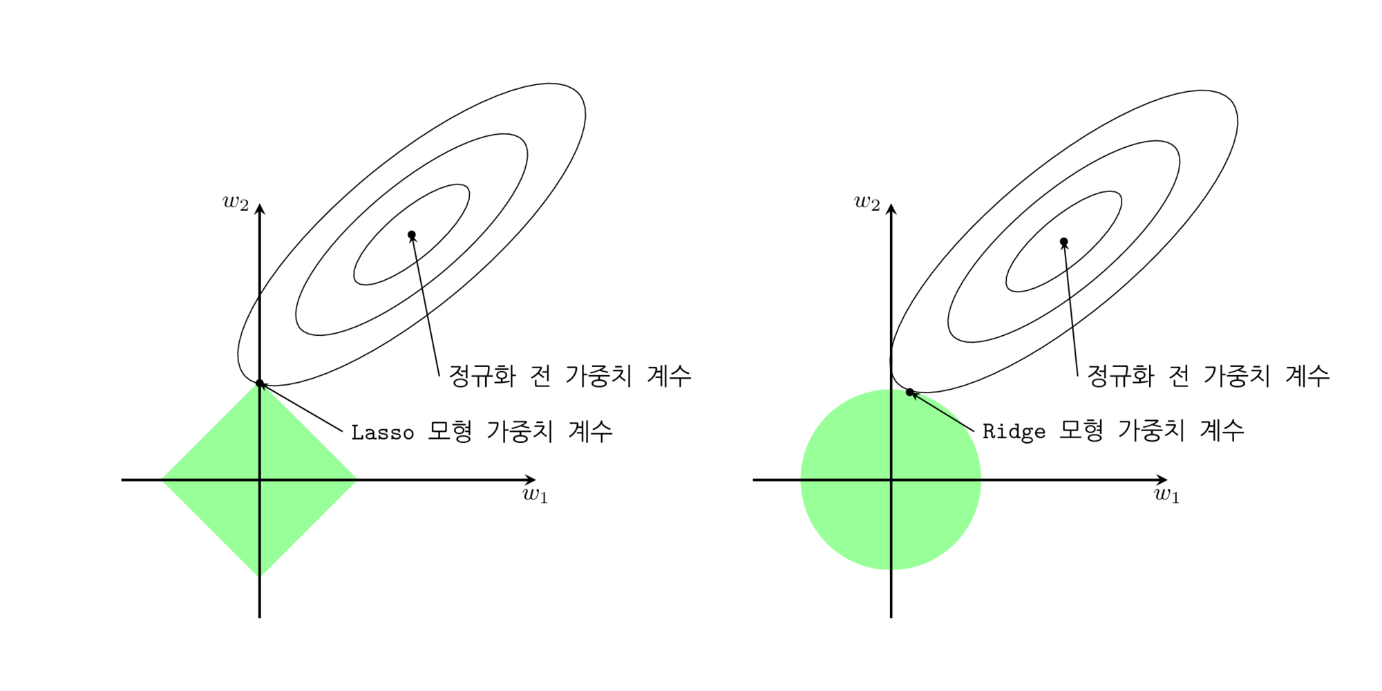
“선형회귀 계수(Weight)에 대한 제약 조건을 추가함으로써 모형이 과도하게 최적화되는 현상, 즉 과최적화를 막는 방법”
“과최적화는 계수 크기를 과도하게 증가하는 경향이 있기에, 정규화 방법에서의 제약 조건은 일반적으로 계수의 크기를 제한하는 방법”
정규화 회귀분석 알고리즘
0) Standard Regression:
1) Ridge Regression:
정규화조건/패널티/제약조건: 추정계수의 제곱합을 최소로 하는 것
\begin{align*} \hat{\beta} = arg\underset{\hat{\beta}}{min} \Biggl[\displaystyle \sum_{j=1}^t \Bigl(y_j - \displaystyle \sum_{i=0}^k \beta_i x_{ij}\Bigr)^2 + \lambda \displaystyle \sum_{i=0}^k \beta_i^2\Biggr] \ where~\lambda~is~hyper~parameter(given~by~human) \end{align*}
하이퍼파라미터(\(\lambda\)): 기존의 잔차 제곱합과 추가 제약 조건의 비중을 조절하기 위한 하이퍼모수(hyperparameter)
\(\lambda\)=0: 일반적인 선형 회귀모형(OLS)
\(\lambda\)를 크게 두면 정규화(패널티) 정도가 커지기 때문에 가중치(\(\beta_i\))의 값들이 커질 수 없음(작아짐)
\(\lambda\)를 작게 두면 정규화(패널티) 정도가 작아 지기 때문에 가중치(\(\beta_i\))의 값들의 자유도가 높아져 커질 수 있음(커짐)
2) Lasso(Least Absolute Shrinkage and Selection Operator) Regression:
정규화조건/패널티/제약조건: 추정계수의 절대값 합을 최소로 하는 것
\begin{align*} \hat{\beta} = arg\underset{\hat{\beta}}{min} \Biggl[\displaystyle \sum_{j=1}^t \Bigl(y_j - \displaystyle \sum_{i=0}^k \beta_i x_{ij}\Bigr)^2 + \lambda \displaystyle \sum_{i=0}^k \left|\beta_i \right|\Biggr] \ where~\lambda~is~hyper~parameter(given~by~human) \end{align*}
3) Elastic Net:
정규화조건/패널티/제약조건: 추정계수의 절대값 합과 제곱합을 동시에 최소로 하는 것
\begin{align*} \hat{\beta} &= arg\underset{\hat{\beta}}{min} \Biggl[\displaystyle \sum_{j=1}^t \Bigl(y_j - \displaystyle \sum_{i=0}^k \beta_i x_{ij}\Bigr)^2 + \lambda_1 \displaystyle \sum_{i=0}^k \left|\beta_i \right| + \lambda_2 \displaystyle \sum_{i=0}^k \beta_i^2\Biggr] \ &where~\lambda_1~and~\lambda_2~are~hyper~parameters(given~by~human) \end{align*}
하이퍼파라미터 특성 및 요약
최적 정규화(최적 하이퍼파라미터 추정): 하이퍼파라미터(Hyperparameter)에 따른 검증성능 차이 존재
Train Set: 하이퍼파라미터가 작으면 작을수록 좋아짐(과최적화)
Test Set: 하이퍼파라미터가 특정한 범위에 있을때 좋아짐(추정필요)
Summary
Standard:
Ridge: - 알고리즘이 모든 변수들을 포함하려 하기 때문에 계수의 크기가 작아지고 모형의 복잡도가 줄어듬
- 모든 변수들을 포함하려 하므로 변수의 수가 많은 경우 효과가 좋지 않으나 과적합(Overfitting)을 방지하는데 효과적
- 다중공선성이 존재할 경우, 변수 간 상관관계에 따라 계수로 다중공선성이 분산되기에 효과가 높음
LASSO:
- 알고리즘이 최소한의 변수를 포함하여 하기 때문의 나머지 변수들의 계수는 0이됨 (Feature Selection 기능)
- 변수선택 기능이 있기에 일반적으로 많이 사용되는 이점이 있지만 특정변수에 대한 계수가 커지는 단점 존재
- 다중공선성이 존재할 경우, 특정 변수만을 선택하는 방식이라 Ridge에 비해 다중공선성 문제에 효과가 낮음
Elastic Net:
- 큰 데이터셋에서 Ridge와 LASSO의 효과를 모두 반영하기에 효과가 좋음 (적은 데이터셋은 효과 낮음)
파라미터 세팅(실습)
1) “statsmodels”: 선형 회귀모형 클래스의 fit_regularized 메서드를 사용하여 Ridge/LASSO/Elastic Net 계수 추정
Ridge:
$\lambda_1 = 0,~~0 < \lambda_2 < 1 \\ => L_1 = 0,~~alpha \ne 0$ - **LASSO:**$0 < \lambda_1 < 1,~~\lambda_2 = 0 \\ => L_1 = 1,~~alpha \ne 0$ - **Elastic Net:**$0 < (\lambda_1, \lambda_2) < 1 \\ => 0 < L_1 < 1,~~alpha \ne 0$ 2) “sklearn”: 정규화 회귀모형을 위한 Ridge, Lasso, ElasticNet 별도 클래스 제공
$0 < (\lambda = alpha) < 1$ - [**LASSO:**](http://scikit-learn.org/stable/modules/generated/sklearn.linear_model.Lasso.html)$0 < (\lambda = alpha) < 1$ - [**Elastic Net:**](http://scikit-learn.org/stable/modules/generated/sklearn.linear_model.ElasticNet.html)$0 < (\lambda_1, \lambda_2) < 1 \\ => 0 < L_1 < 1,~~alpha \ne 0$
# Ridge
fit = Ridge(alpha=0.5, fit_intercept=True, normalize=True, random_state=123).fit(X_train, Y_train)
pred_tr = fit.predict(X_train)
pred_te = fit.predict(X_test)
# LASSO
fit = Lasso(alpha=0.5, fit_intercept=True, normalize=True, random_state=123).fit(X_train, Y_train)
pred_tr = fit.predict(X_train)
pred_te = fit.predict(X_test)
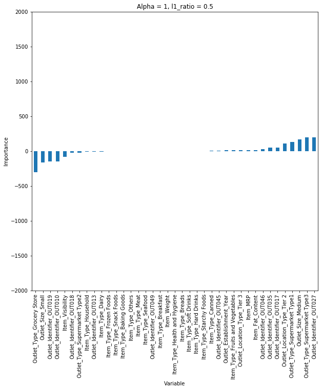
# Elastic Net
fit = ElasticNet(alpha=0.01, l1_ratio=1, fit_intercept=True, normalize=True, random_state=123).fit(X_train, Y_train)
pred_tr = fit.predict(X_train)
pred_te = fit.predict(X_test)
실습
import warnings
warnings.filterwarnings('always')
warnings.filterwarnings('ignore')
import pandas as pd
import numpy as np
from sklearn import datasets
import matplotlib.pyplot as plt
from sklearn.linear_model import Ridge, Lasso, ElasticNet
diabetes = datasets.load_diabetes()
X = diabetes.data
y = diabetes.target
print('Data View')
display(pd.concat([pd.DataFrame(y, columns=['diabetes_value']), pd.DataFrame(X, columns=diabetes.feature_names)], axis=1).head())
Data View
| diabetes_value | age | sex | bmi | bp | s1 | s2 | s3 | s4 | s5 | s6 | |
|---|---|---|---|---|---|---|---|---|---|---|---|
| 0 | 151.0 | 0.038076 | 0.050680 | 0.061696 | 0.021872 | -0.044223 | -0.034821 | -0.043401 | -0.002592 | 0.019908 | -0.017646 |
| 1 | 75.0 | -0.001882 | -0.044642 | -0.051474 | -0.026328 | -0.008449 | -0.019163 | 0.074412 | -0.039493 | -0.068330 | -0.092204 |
| 2 | 141.0 | 0.085299 | 0.050680 | 0.044451 | -0.005671 | -0.045599 | -0.034194 | -0.032356 | -0.002592 | 0.002864 | -0.025930 |
| 3 | 206.0 | -0.089063 | -0.044642 | -0.011595 | -0.036656 | 0.012191 | 0.024991 | -0.036038 | 0.034309 | 0.022692 | -0.009362 |
| 4 | 135.0 | 0.005383 | -0.044642 | -0.036385 | 0.021872 | 0.003935 | 0.015596 | 0.008142 | -0.002592 | -0.031991 | -0.046641 |
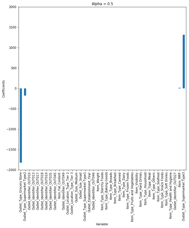
alpha_weight = 0.5
fit = Ridge(alpha=alpha_weight, fit_intercept=True, normalize=True, random_state=123).fit(X, y)
pd.DataFrame(np.hstack([fit.intercept_, fit.coef_]), columns=['alpha = {}'.format(alpha_weight)])
| alpha = 0.5 | |
|---|---|
| 0 | 152.133484 |
| 1 | 20.137357 |
| 2 | -131.242606 |
| 3 | 383.481783 |
| 4 | 244.837872 |
| 5 | -15.187056 |
| 6 | -58.344798 |
| 7 | -174.842798 |
| 8 | 121.985055 |
| 9 | 328.499702 |
| 10 | 110.886036 |
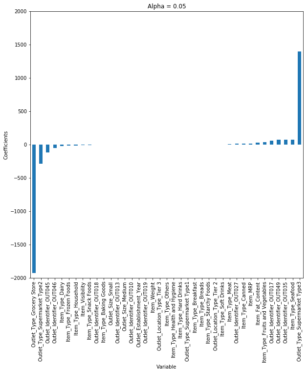
alpha_weight = 0.5
fit = Lasso(alpha=alpha_weight, fit_intercept=True, normalize=True, random_state=123).fit(X, y)
pd.DataFrame(np.hstack([fit.intercept_, fit.coef_]), columns=['alpha = {}'.format(alpha_weight)])
| alpha = 0.5 | |
|---|---|
| 0 | 152.133484 |
| 1 | 0.000000 |
| 2 | -0.000000 |
| 3 | 471.038733 |
| 4 | 136.507108 |
| 5 | -0.000000 |
| 6 | -0.000000 |
| 7 | -58.319549 |
| 8 | 0.000000 |
| 9 | 408.023324 |
| 10 | 0.000000 |
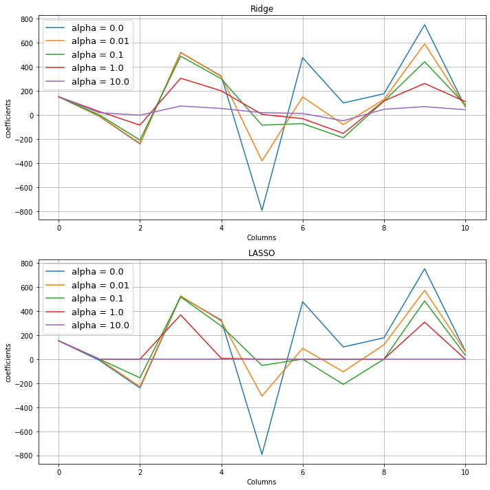
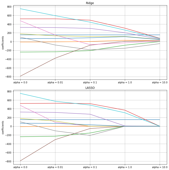
result_Ridge = pd.DataFrame()
alpha_candidate = np.hstack([0, np.logspace(-2, 1, 4)])
for alpha_weight in alpha_candidate:
    fit = Ridge(alpha=alpha_weight, fit_intercept=True, normalize=True, random_state=123).fit(X, y)
    result_coef = pd.DataFrame(np.hstack([fit.intercept_, fit.coef_]), columns=['alpha = {}'.format(alpha_weight)])
    result_Ridge = pd.concat([result_Ridge, result_coef], axis=1)

result_LASSO = pd.DataFrame()
alpha_candidate = np.hstack([0, np.logspace(-2, 1, 4)])
for alpha_weight in alpha_candidate:
    fit = Lasso(alpha=alpha_weight, fit_intercept=True, normalize=True, random_state=123).fit(X, y)
    result_coef = pd.DataFrame(np.hstack([fit.intercept_, fit.coef_]), columns=['alpha = {}'.format(alpha_weight)])
    result_LASSO = pd.concat([result_LASSO, result_coef], axis=1)

result_Ridge.plot(figsize=(10,10), legend=True, ax=plt.subplot(211))
plt.title('Ridge')
plt.xlabel('Columns')
plt.ylabel('coefficients')
plt.legend(fontsize=13)
plt.grid()
result_LASSO.plot(legend=True, ax=plt.subplot(212))
plt.title('LASSO')
plt.xlabel('Columns')
plt.ylabel('coefficients')
plt.legend(fontsize=13)
plt.tight_layout()
plt.grid()
plt.show()
result_Ridge.T.plot(figsize=(10,10), legend=False, ax=plt.subplot(211))
plt.title('Ridge')
plt.xticks(np.arange(len(result_Ridge.columns)), [i for i in result_Ridge.columns])
plt.ylabel('coefficients')
plt.grid()
result_LASSO.T.plot(legend=False, ax=plt.subplot(212))
plt.title('LASSO')
plt.xticks(np.arange(len(result_Ridge.columns)), [i for i in result_Ridge.columns])
plt.ylabel('coefficients')
plt.tight_layout()
plt.grid()
plt.show()
Bagging and Boosting 모델
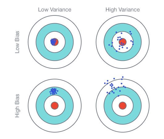
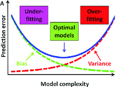
편향-분산 상충관계(Bias-variance Trade-off)
1) 편향과 분산의 정의
(비수학적 이해)
편향(Bias): 점추정
예측값과 실제값의 차이
모델 학습시 여러 데이터로 학습 후 예측값의 범위가 정답과 얼마나 멀리 있는지 측정
편향(Bias(Real)): 모형화(단순화)로 미처 반영하지 못한 복잡성
=> 편향이 작다면 Training 데이터 패턴(복잡성)을 최대반영 의미
=> 편향이 크다면 Training 데이터 패턴(복잡성)을 최소반영 의미분산(Variance): 구간추정
학습한 모델의 예측값이 평균으로부터 퍼진 정도(변동성/분산)
여러 모델로 학습을 반복한다면, 학습된 모델별로 예측한 값들의 차이를 측정
분산(Variance(Real)): 다른 데이터(Testing)를 사용했을때 발생할 변화
=> 분산이 작다면 다른 데이터로 예측시 적은 변동 예상
=> 분산이 크다면 다른 데이터로 예측시 많은 변동 예상
(수학적 이해)
\begin{align*} \text{Equation of Error} && Err(x) &= E\Bigl[\bigl(Y-\hat{f}(x)\bigr)^2 \Bigr] \ && &= \Bigl(E[\hat{f}(x)] - f(x)\Bigr)^2 + E \Bigl[\bigl(\hat{f}(x) - E[\hat{f}(x)]\bigr)^2 \Bigr] + \sigma_{\epsilon}^2 \ && &= \text{Bias}^2 + \text{Variance} + \text{Irreducible Error} \end{align*}
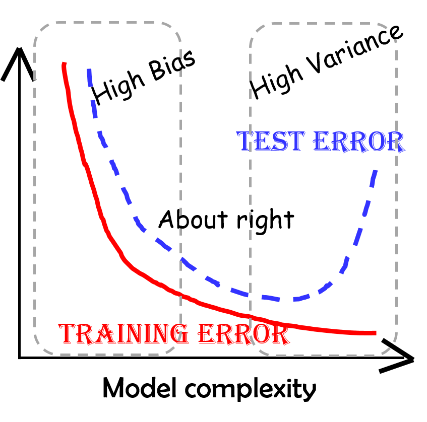
2) 편향과 분산의 관계
모델의 복잡도가 낮으면 Bias가 증가하고 Variance가 감소(Underfitting)
: 구간추정 범위는 좁으나 점추정 정확성 낮음
: Training/Testing 모두 예측력이 낮음모델의 복잡도가 높으면 Bias가 감소하고 Variance가 증가(Overfitting)
: 점추정 정확성은 높으나 구간추정 범위는 넓음
: Training만 잘 예측력 높고 Testing은 예측력 낮음Bias와 Variance가 최소화 되는 수준에서 모델의 복잡도 선택
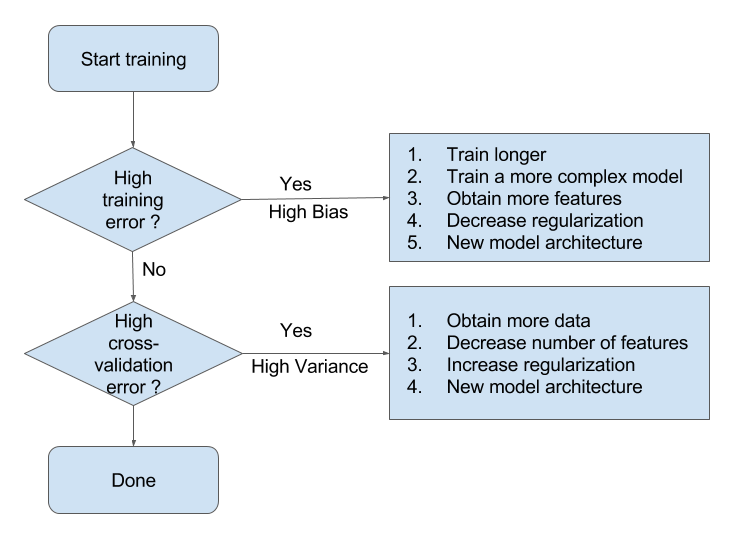
3) 편향과 분산 모두를 최소화하는 방법
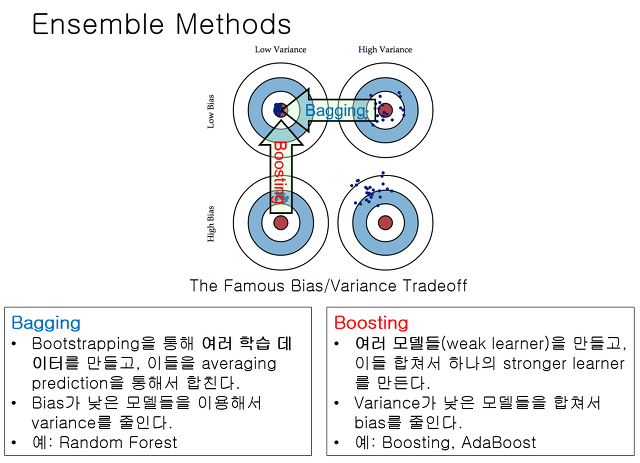
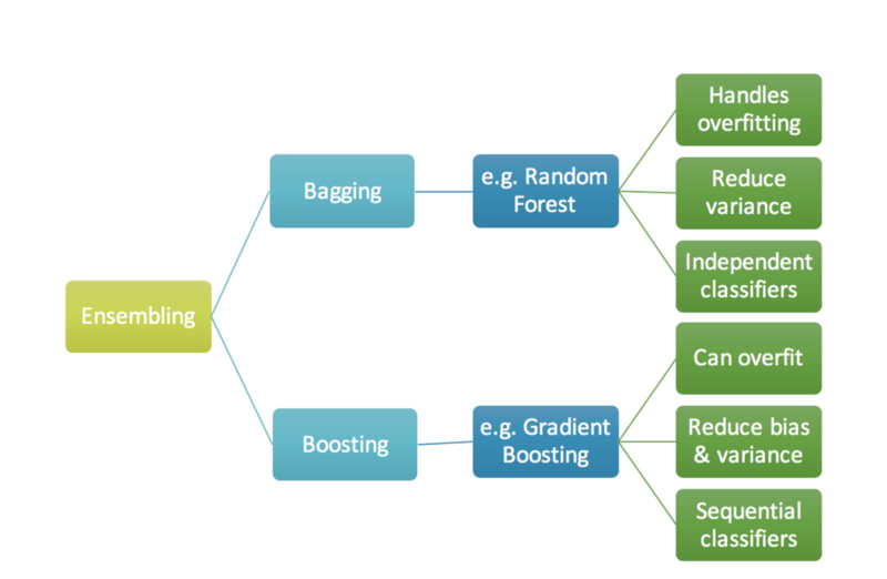
Bagging vs Boosting
앙상블(Ensemble, Ensemble Learning, Ensemble Method)이란 머신러닝에서 여러개의 모델을 학습시켜,
그 모델들의 예측결과들을 이용해 하나의 모델보다 더 나은 값을 예측하는 방법
Bagging(Bootstrap Aggregating):
부트스트래핑(Bootstraping): 예측값과 실제값의 차이 중복을 허용한 리샘플링(Resampling)
페이스팅(Pasting): 이와 반대로 중복을 허용하지 않는 샘플링
Boosting:
성능이 약한 학습기(weak learner)를 여러 개 연결하여 강한 학습기(strong learner)를 만드는 앙상블 학습
앞에서 학습된 모델을 보완해나가면서 더나은 모델로 학습시키는 것
- |
Bagging |
Boosting |
|---|---|---|
특징 |
병렬 앙상블 모델(각 모델은 서로 독립) |
연속 앙상블 모델(이전 모델의 오류 반영) |
목적 |
Variance 감소 |
Bias 감소 |
적합한 상황 |
Low Bias + High Variance |
High Bias + Low Variance |
Sampling |
Random Sampling |
Random Sampling with weight on error |
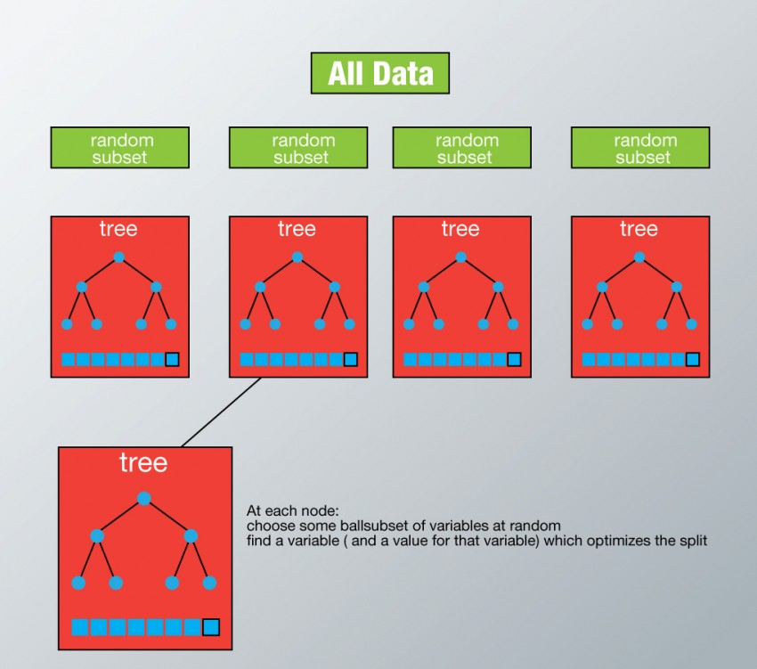
Bagging 알고리즘
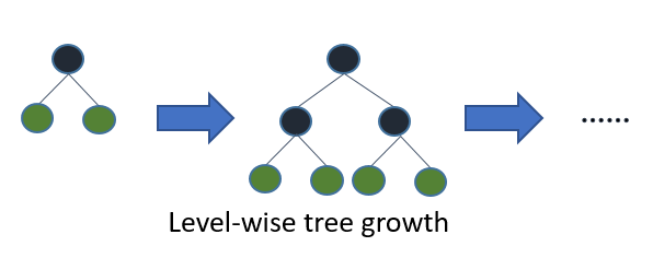
의사결정나무(Decision Tree):
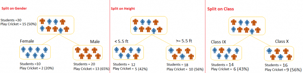
렌덤포레스트(Random Forest): 여러개의 의사결정나무(Decision Tree) 생성한 다음, 각 개별 트리의 예측값들 중 가장 많은 선택을 받은 변수들로 예측하는 알고리즘, 의사결정나무의 CLT버전
# DecisionTree
fit = DecisionTreeRegressor().fit(X_train, Y_train)
pred_tr = fit.predict(X_train)
pred_te = fit.predict(X_test)

# RandomForestRegressor
fit = RandomForestRegressor(n_estimators=100, random_state=123).fit(X_train, Y_train)
pred_tr = fit.predict(X_train)
pred_te = fit.predict(X_test)
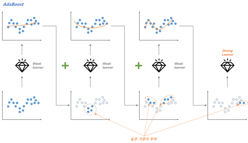
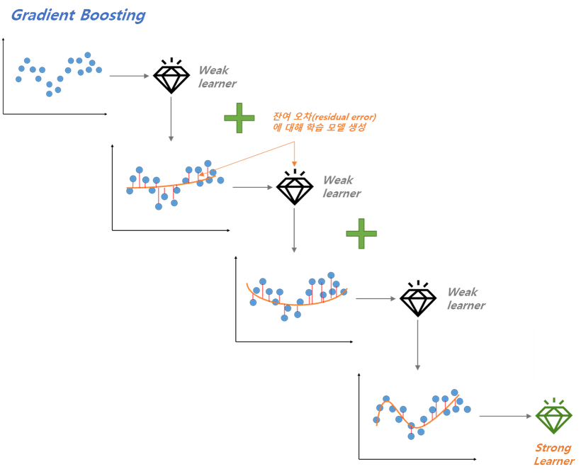
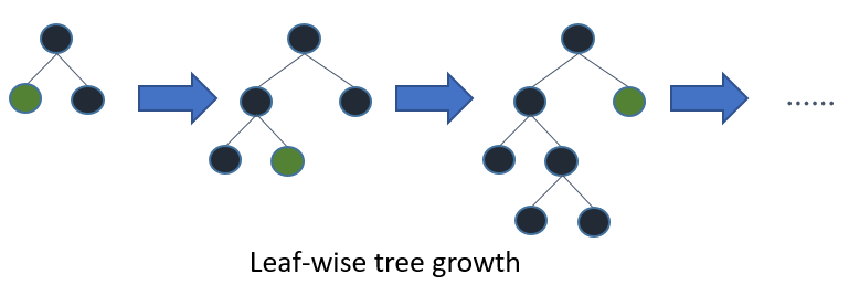
Boosting 알고리즘
Adaptive Boosting(AdaBoost): 학습된 모델이 과소적합(학습하기 어려운 데이터)된 학습 데이터 샘플의 가중치를 높이면서 더 잘 적합되도록 하는 방식
Gradient Boosting Machine(GBM): 아다부스트 처럼 학습단계 마다 데이터 샘플의 가중치를 업데이트 하는 것이 아니라, 학습 전단계 모델에서의 잔차(Residual)을 모델에 학습시키는 방법
XGBoost(eXtreme Gradient Boosting): 높은 예측력으로 많은 양의 데이터를 다룰 때 사용되는 부스팅 알고리즘
LightGBM: 현존하는 부스팅 알고리즘 중 가장 빠르고 높은 예측력 제공
Algorithms |
Specification |
Others |
|---|---|---|
AdaBoost |
다수결을 통한 정답분류 및 오답에 가중치 부여 |
- |
GBM |
손실함수(검증지표)의 Gradient로 오답에 가중치 부여 |
- |
XGBoost |
GMB대비 성능향상 |
2014년 공개 |
LightGBM |
XGBoost대비 성능향상 및 자원소모 최소화 |
2016년 공개 |
# GradientBoostingRegression
fit = GradientBoostingRegressor(alpha=0.1, learning_rate=0.05, loss='huber', criterion='friedman_mse',
                                           n_estimators=1000, random_state=123).fit(X_train, Y_train)
pred_tr = fit.predict(X_train)
pred_te = fit.predict(X_test)

# XGBoost
fit = XGBRegressor(learning_rate=0.05, n_estimators=100, random_state=123).fit(X_train, Y_train)
pred_tr = fit.predict(X_train)
pred_te = fit.predict(X_test)

# LightGMB
fit = LGBMRegressor(learning_rate=0.05, n_estimators=100, random_state=123).fit(X_train, Y_train)
pred_tr = fit.predict(X_train)
pred_te = fit.predict(X_test)
비교
시계열 알고리즘
비정상성(Non-stationary)의 정상성(Stationary) 변환
목적: 정상성 확보를 통해 안정성이 높아지고 예측력 향상
장점: 절약성 원칙(Principle of Parsimony)에 따라 적은 모수만으로 모델링 가능하기에 과적합 확률이 줄어듬
방법: 제곱, 루트, 로그, 차분 등
이론예시:
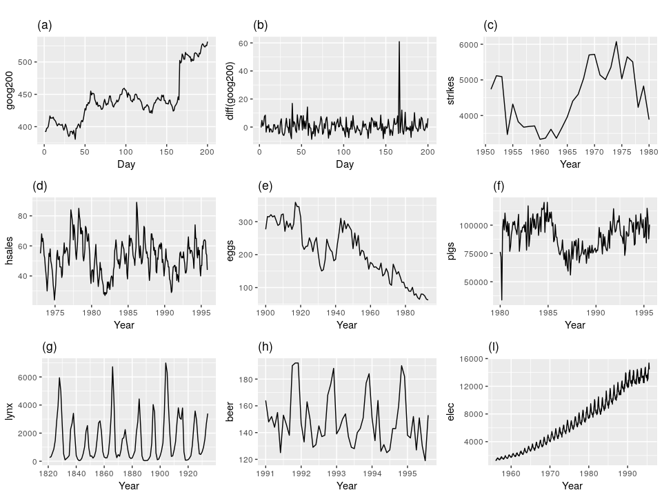
- Trend: a/c/e/f/i
- Seasonality: d/h/i
- Cycle: g
- Non-constant Variance: i
1) 로그변환(Logarithm Transform):
시간흐름에 비례하여 값이 커지는 경우(분산 증가)
비정상 확률 과정으로 표준편차가 자료의 크기에 비례하여 증가하거나 지수함수적으로 증가하는 경우
로그 변환한 확률 과정의 분산은 일정하기에 추세 제거로 기댓값이 0이 되면 정상 과정으로 모형화 가능
\begin{align*} \text{Distribution of Original} && \text{E}(Y_t) &= \mu_t = f(t) \ && \sqrt{\text{Var}(Y_t)} &= \mu_t \sigma \ \text{Distribution of Log-transform} && Y_t &= Y_{t-1} + Y_t - Y_{t-1} \ && \dfrac{Y_t}{Y_{t-1}} &= 1 + \dfrac{Y_t - Y_{t-1}}{Y_{t-1}} \ && log(\dfrac{Y_t}{Y_{t-1}}) &= log(1 + \dfrac{Y_t - Y_{t-1}}{Y_{t-1}}) \approx \dfrac{Y_t - Y_{t-1}}{Y_{t-1}} \ && log(Y_t) - log(Y_{t-1}) &\approx \dfrac{Y_t - Y_{t-1}}{Y_{t-1}} \ && log(Y_t) &\approx log(Y_{t-1}) + \dfrac{Y_t - Y_{t-1}}{Y_{t-1}} \ && log(Y_t) &\approx log(\mu_t) + \dfrac{Y_t - \mu_t}{\mu_t} \ && \text{E}(\log Y_t) &= \log \mu_t \ && \text{Var}(\log Y_t) &\approx \sigma^2 \ \text{Generalization of Return} && R_t &= \dfrac{Y_{t}}{Y_{t-1}} - 1 \ && \log{Y_t} - \log{Y_{t-1}} &= \log{R_t + 1} \approx R_t ;; \text{ if } \left| R_t \right| < 0.2 \ \end{align}
2) 차분(Difference): 특정 시점 또는 시점들의 데이터가 발산할 경우 시점간 차분(변화량)으로 정상성 변환 가능
계절성(Seasonality, \(S_t\)): 특정한 달/요일에 따라 기대값이 달라지는 것, 변수 더미화를 통해 추정 가능
계절성 제거: 1) 계절성 추정(\(f(t)\)) 후 계절성 제거를 통한 정상성 확보 (수학적 이해) - 확률과정의 계절변수 더미화를 통해 기댓값 함수를 알아내는 것 - 확률과정(\(Y_t\))이 추정이 가능한 결정론적 계절성함수(\(f(t)\))와 정상확률과정(\(Y^s_t\))의 합
\begin{align*}
\text{Main Equation} && Y_t &= f(t) + Y^s_t \\
\text{where} && f(t) &= \sum_{i=0}^{\infty} a_i D_i = a_0 + a_1 D_1 + a_2 D_2 + \cdots
\end{align*}
계절성 제거: 2) 차분 적용 \((1-L^d) Y_t\) 후 계절성 제거를 통한 정상성 확보 (수학적 이해)
\begin{align*}
\text{Main Equation of d=1} && Y_t &=> (1-L^1) Y_t \\
&& &= (1-Lag^1) Y_t \\
&& &= Y_t - Lag^1(Y_t) \\
&& &= Y_t - Y_{t-1} \\
\text{Main Equation of d=2} && Y_t &=> (1-L^2) Y_t \\
&& &= (1-Lag^2) Y_t \\
&& &= Y_t - Lag^2(Y_t) \\
&& &= Y_t - Y_{t-2} \\
\end{align*}
추세(Trend, \(T_t\)): 시계열이 시간에 따라 증가, 감소 또는 일정 수준을 유지하는 경우
추세 제거: 1) 추세 추정(\(f(t)\)) 후 추세 제거를 통한 정상성 확보 (수학적 이해) - 확률과정의 결정론적 기댓값 함수를 알아내는 것 - 확률과정(\(Y_t\))이 추정이 가능한 결정론적 추세함수(\(f(t)\))와 정상확률과정(\(Y^s_t\))의 합
\begin{align*}
\text{Main Equation} && Y_t &= f(t) + Y^s_t \\
\text{where} && f(t) &= \sum_{i=0}^{\infty} a_i t^i = a_0 + a_1 t + a_2 t^2 + \cdots
\end{align*}
추세 제거: 2) 차분 적용 \((1-L^1)^d Y_t\) 후 추세 제거를 통한 정상성 확보 (수학적 이해)
\begin{align*}
\text{Main Equation of d=1} && Y_t &=> (1-L^1)^1 Y_t \\
&& &= (1-Lag^1)^1 Y_t \\
&& &= Y_t - Lag^1(Y_t) \\
&& &= Y_t - Y_{t-1} \\
\text{Main Equation of d=2} && Y_t &=> (1-L^1)^2 Y_t \\
&& &= (1-2L^1+L^2) Y_t \\
&& &= (1-2Lag^1+Lag^2) Y_t \\
&& &= Y_t - 2Lag^1(Y_t) + Lag^2(Y_t) \\
&& &= Y_t - Lag^1(Y_t) - Lag^1(Y_t) + Lag^2(Y_t) \\
&& &= (Y_t - Lag^1(Y_t)) - (Lag^1(Y_t) - Lag^2(Y_t)) \\
&& &= (Y_t - L^1(Y_t)) - (L^1(Y_t) - L^2(Y_t)) \\
&& &= (Y_t - Y_{t-1}) - (Y_{t-1} - Y_{t-2}) \\
&& &= Y_t - 2Y_{t-1} + Y_{t-2} \\
\end{align*}
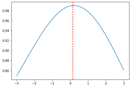
3) Box-Cox 변환: 정규분포가 아닌 자료를 정규분포로 변환하기 위해 사용
모수(parameter) \(\lambda\)를 가지며, 보통 여러가지 \(\lambda\) 값을 시도하여 가장 정규성을 높여주는 값을 사용
\begin{align*} y^{(\boldsymbol{\lambda})} = \begin{cases} \dfrac{y^{\lambda} - 1}{\lambda} & \text{if } \lambda \neq 0, \ \ln{y} & \text{if } \lambda = 0, \end{cases} \end{align*}
정상성 테스트 방향
추세와 계절성 모두 제거된 정상성 데이터 변환 필요!
ADF 정상성 확인 -> 추세 제거 확인 Measure
: ADF 검정통계량은 정상이라고 해도 데이터에 계절성이 포함되면 ACF의 비정상 Lag 존재하는 비정상데이터 가능
KPSS 정상성 확인 -> 계절성 제거 확인 Measure
: KPSS 검정통계량은 정상이라고 해도 데이터에 추세가 포함되면 ACF의 비정상 Lag 존재하는 비정상데이터 가능
실습: 대기중 CO2농도 추세 제거
# 라이브러리 및 데이터 로딩
import pandas as pd
from statsmodels import datasets
import matplotlib.pyplot as plt
import statsmodels.api as sm
%reload_ext autoreload
%autoreload 2
from module import stationarity_adf_test, stationarity_kpss_test

raw_set = datasets.get_rdataset("CO2", package="datasets")
raw = raw_set.data
---------------------------------------------------------------------------
ModuleNotFoundError                       Traceback (most recent call last)
<ipython-input-7-c1948bb6176f> in <module>
      6 get_ipython().run_line_magic('reload_ext', 'autoreload')
      7 get_ipython().run_line_magic('autoreload', '2')
----> 8 from module import stationarity_adf_test, stationarity_kpss_test
      9
     10 raw_set = datasets.get_rdataset("CO2", package="datasets")

ModuleNotFoundError: No module named 'module'
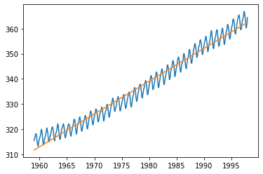
# 데이터 확인 및 추세 추정 (선형)
display(raw.head())
plt.plot(raw.time, raw.value)
plt.show()

result = sm.OLS.from_formula(formula='value~time', data=raw).fit()
display(result.summary())

trend = result.params[0] + result.params[1] * raw.time
plt.plot(raw.time, raw.value, raw.time, trend)
plt.show()
| time | value | |
|---|---|---|
| 0 | 1,959.00 | 315.42 |
| 1 | 1,959.08 | 316.31 |
| 2 | 1,959.17 | 316.50 |
| 3 | 1,959.25 | 317.56 |
| 4 | 1,959.33 | 318.13 |

| Dep. Variable: | value | R-squared: | 0.969 |
|---|---|---|---|
| Model: | OLS | Adj. R-squared: | 0.969 |
| Method: | Least Squares | F-statistic: | 1.479e+04 |
| Date: | Fri, 31 Jul 2020 | Prob (F-statistic): | 0.00 |
| Time: | 22:45:19 | Log-Likelihood: | -1113.5 |
| No. Observations: | 468 | AIC: | 2231. |
| Df Residuals: | 466 | BIC: | 2239. |
| Df Model: | 1 | ||
| Covariance Type: | nonrobust |
| coef | std err | t | P>|t| | [0.025 | 0.975] | |
|---|---|---|---|---|---|---|
| Intercept | -2249.7742 | 21.268 | -105.784 | 0.000 | -2291.566 | -2207.982 |
| time | 1.3075 | 0.011 | 121.634 | 0.000 | 1.286 | 1.329 |
| Omnibus: | 15.857 | Durbin-Watson: | 0.212 |
|---|---|---|---|
| Prob(Omnibus): | 0.000 | Jarque-Bera (JB): | 7.798 |
| Skew: | 0.048 | Prob(JB): | 0.0203 |
| Kurtosis: | 2.375 | Cond. No. | 3.48e+05 |
Warnings:
[1] Standard Errors assume that the covariance matrix of the errors is correctly specified.
[2] The condition number is large, 3.48e+05. This might indicate that there are
strong multicollinearity or other numerical problems.
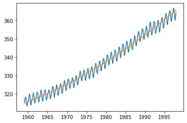
# 데이터 확인 및 추세 추정 (비선형)
display(raw.head())
plt.plot(raw.time, raw.value)
plt.show()

result = sm.OLS.from_formula(formula='value~time+I(time**2)', data=raw).fit()
display(result.summary())

trend = result.params[0] + result.params[1] * raw.time + result.params[2] * raw.time**2
plt.plot(raw.time, raw.value, raw.time, trend)
plt.show()
| time | value | |
|---|---|---|
| 0 | 1,959.00 | 315.42 |
| 1 | 1,959.08 | 316.31 |
| 2 | 1,959.17 | 316.50 |
| 3 | 1,959.25 | 317.56 |
| 4 | 1,959.33 | 318.13 |

| Dep. Variable: | value | R-squared: | 0.979 |
|---|---|---|---|
| Model: | OLS | Adj. R-squared: | 0.979 |
| Method: | Least Squares | F-statistic: | 1.075e+04 |
| Date: | Fri, 31 Jul 2020 | Prob (F-statistic): | 0.00 |
| Time: | 22:45:20 | Log-Likelihood: | -1027.8 |
| No. Observations: | 468 | AIC: | 2062. |
| Df Residuals: | 465 | BIC: | 2074. |
| Df Model: | 2 | ||
| Covariance Type: | nonrobust |
| coef | std err | t | P>|t| | [0.025 | 0.975] | |
|---|---|---|---|---|---|---|
| Intercept | 4.77e+04 | 3482.902 | 13.696 | 0.000 | 4.09e+04 | 5.45e+04 |
| time | -49.1907 | 3.521 | -13.971 | 0.000 | -56.110 | -42.272 |
| I(time ** 2) | 0.0128 | 0.001 | 14.342 | 0.000 | 0.011 | 0.015 |
| Omnibus: | 66.659 | Durbin-Watson: | 0.306 |
|---|---|---|---|
| Prob(Omnibus): | 0.000 | Jarque-Bera (JB): | 17.850 |
| Skew: | -0.116 | Prob(JB): | 0.000133 |
| Kurtosis: | 2.072 | Cond. No. | 1.35e+11 |
Warnings:
[1] Standard Errors assume that the covariance matrix of the errors is correctly specified.
[2] The condition number is large, 1.35e+11. This might indicate that there are
strong multicollinearity or other numerical problems.
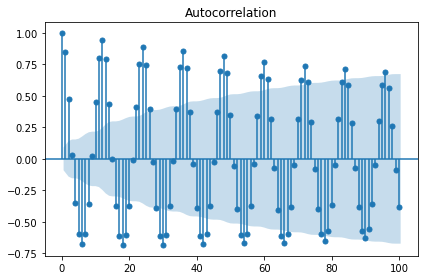
# 추세 제거 및 정상성 확인
## 방법1
plt.plot(raw.time, result.resid)
plt.show()

display(stationarity_adf_test(result.resid, []))
display(stationarity_kpss_test(result.resid, []))

sm.graphics.tsa.plot_acf(result.resid, lags=100, use_vlines=True)
plt.tight_layout()
plt.show()

| Stationarity_adf | |
|---|---|
| Test Statistics | -2.53 |
| p-value | 0.11 |
| Used Lag | 13.00 |
| Used Observations | 454.00 |
| Critical Value(1%) | -3.44 |
| Maximum Information Criteria | 260.10 |
| Stationarity_kpss | |
|---|---|
| Test Statistics | 0.17 |
| p-value | 0.10 |
| Used Lag | 18.00 |
| Critical Value(10%) | 0.35 |
# 추세 제거 및 정상성 확인
## 방법2
plt.plot(raw.time[1:], raw.value.diff(1).dropna())
plt.show()

display(stationarity_adf_test(raw.value.diff(1).dropna(), []))
display(stationarity_kpss_test(raw.value.diff(1).dropna(), []))

sm.graphics.tsa.plot_acf(raw.value.diff(1).dropna(), lags=100, use_vlines=True)
plt.tight_layout()
plt.show()
| Stationarity_adf | |
|---|---|
| Test Statistics | -5.14 |
| p-value | 0.00 |
| Used Lag | 12.00 |
| Used Observations | 454.00 |
| Critical Value(1%) | -3.44 |
| Maximum Information Criteria | 271.87 |
| Stationarity_kpss | |
|---|---|
| Test Statistics | 0.04 |
| p-value | 0.10 |
| Used Lag | 18.00 |
| Critical Value(10%) | 0.35 |
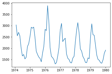
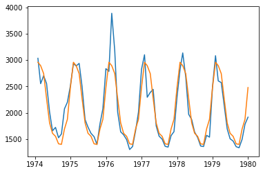
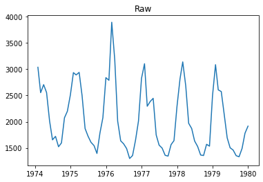
실습: 호흡기질환 사망자수 계절성 제거
# 라이브러리 및 데이터 로딩
import pandas as pd
from statsmodels import datasets
import matplotlib.pyplot as plt
import statsmodels.api as sm
%reload_ext autoreload
%autoreload 2
from module import stationarity_adf_test, stationarity_kpss_test

raw_set = datasets.get_rdataset("deaths", package="MASS")
raw = raw_set.data
# 시간변수 추출
raw.time = pd.date_range('1974-01-01', periods=len(raw), freq='M')
raw['month'] = raw.time.dt.month
# 데이터 확인 및 추세 추정
display(raw.tail())
plt.plot(raw.time, raw.value)
plt.show()

display(stationarity_adf_test(raw.value, []))
display(stationarity_kpss_test(raw.value, []))
sm.graphics.tsa.plot_acf(raw.value, lags=50, use_vlines=True, title='ACF')
plt.tight_layout()
plt.show()

result = sm.OLS.from_formula(formula='value ~ C(month) - 1', data=raw).fit()
display(result.summary())

plt.plot(raw.time, raw.value, raw.time, result.fittedvalues)
plt.show()
| time | value | month | |
|---|---|---|---|
| 67 | 1979-08-31 | 1354 | 8 |
| 68 | 1979-09-30 | 1333 | 9 |
| 69 | 1979-10-31 | 1492 | 10 |
| 70 | 1979-11-30 | 1781 | 11 |
| 71 | 1979-12-31 | 1915 | 12 |
| Stationarity_adf | |
|---|---|
| Test Statistics | -0.57 |
| p-value | 0.88 |
| Used Lag | 12.00 |
| Used Observations | 59.00 |
| Critical Value(1%) | -3.55 |
| Maximum Information Criteria | 841.38 |
| Stationarity_kpss | |
|---|---|
| Test Statistics | 0.65 |
| p-value | 0.02 |
| Used Lag | 12.00 |
| Critical Value(10%) | 0.35 |
| Dep. Variable: | value | R-squared: | 0.853 |
|---|---|---|---|
| Model: | OLS | Adj. R-squared: | 0.826 |
| Method: | Least Squares | F-statistic: | 31.66 |
| Date: | Fri, 31 Jul 2020 | Prob (F-statistic): | 6.55e-21 |
| Time: | 22:45:23 | Log-Likelihood: | -494.38 |
| No. Observations: | 72 | AIC: | 1013. |
| Df Residuals: | 60 | BIC: | 1040. |
| Df Model: | 11 | ||
| Covariance Type: | nonrobust |
| coef | std err | t | P>|t| | [0.025 | 0.975] | |
|---|---|---|---|---|---|---|
| C(month)[1] | 2959.3333 | 103.831 | 28.502 | 0.000 | 2751.641 | 3167.025 |
| C(month)[2] | 2894.6667 | 103.831 | 27.879 | 0.000 | 2686.975 | 3102.359 |
| C(month)[3] | 2743.0000 | 103.831 | 26.418 | 0.000 | 2535.308 | 2950.692 |
| C(month)[4] | 2269.6667 | 103.831 | 21.859 | 0.000 | 2061.975 | 2477.359 |
| C(month)[5] | 1805.1667 | 103.831 | 17.386 | 0.000 | 1597.475 | 2012.859 |
| C(month)[6] | 1608.6667 | 103.831 | 15.493 | 0.000 | 1400.975 | 1816.359 |
| C(month)[7] | 1550.8333 | 103.831 | 14.936 | 0.000 | 1343.141 | 1758.525 |
| C(month)[8] | 1408.3333 | 103.831 | 13.564 | 0.000 | 1200.641 | 1616.025 |
| C(month)[9] | 1397.3333 | 103.831 | 13.458 | 0.000 | 1189.641 | 1605.025 |
| C(month)[10] | 1690.0000 | 103.831 | 16.277 | 0.000 | 1482.308 | 1897.692 |
| C(month)[11] | 1874.0000 | 103.831 | 18.049 | 0.000 | 1666.308 | 2081.692 |
| C(month)[12] | 2478.5000 | 103.831 | 23.871 | 0.000 | 2270.808 | 2686.192 |
| Omnibus: | 19.630 | Durbin-Watson: | 1.374 |
|---|---|---|---|
| Prob(Omnibus): | 0.000 | Jarque-Bera (JB): | 49.630 |
| Skew: | 0.787 | Prob(JB): | 1.67e-11 |
| Kurtosis: | 6.750 | Cond. No. | 1.00 |
Warnings:
[1] Standard Errors assume that the covariance matrix of the errors is correctly specified.
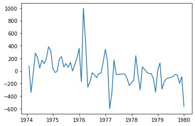
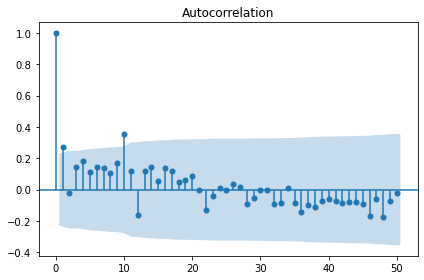
# 추세 제거 및 정상성 확인
## 방법1
plt.plot(raw.time, result.resid)
plt.show()

display(stationarity_adf_test(result.resid, []))
display(stationarity_kpss_test(result.resid, []))
sm.graphics.tsa.plot_acf(result.resid, lags=50, use_vlines=True)
plt.tight_layout()
plt.show()
| Stationarity_adf | |
|---|---|
| Test Statistics | -5.84 |
| p-value | 0.00 |
| Used Lag | 0.00 |
| Used Observations | 71.00 |
| Critical Value(1%) | -3.53 |
| Maximum Information Criteria | 812.36 |
| Stationarity_kpss | |
|---|---|
| Test Statistics | 0.54 |
| p-value | 0.03 |
| Used Lag | 12.00 |
| Critical Value(10%) | 0.35 |
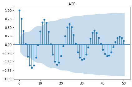
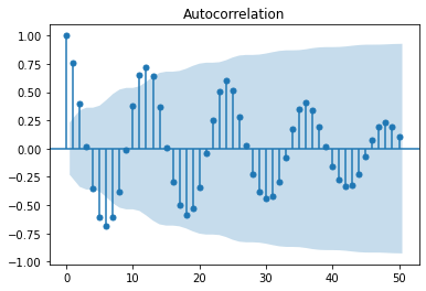
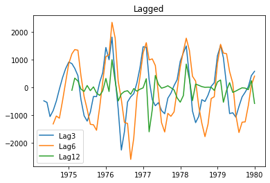
# 계절성 제거 및 정상성 확인
## 방법2
sm.graphics.tsa.plot_acf(raw.value, lags=50, use_vlines=True)
plt.show()
plt.plot(raw.time, raw.value)
plt.title('Raw')
plt.show()
seasonal_lag = 3
plt.plot(raw.time[seasonal_lag:], raw.value.diff(seasonal_lag).dropna(), label='Lag{}'.format(seasonal_lag))
seasonal_lag = 6
plt.plot(raw.time[seasonal_lag:], raw.value.diff(seasonal_lag).dropna(), label='Lag{}'.format(seasonal_lag))
seasonal_lag = 12
plt.plot(raw.time[seasonal_lag:], raw.value.diff(seasonal_lag).dropna(), label='Lag{}'.format(seasonal_lag))
plt.title('Lagged')
plt.legend()
plt.show()
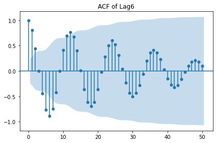
seasonal_lag = 6
display(stationarity_adf_test(raw.value.diff(seasonal_lag).dropna(), []))
display(stationarity_kpss_test(raw.value.diff(seasonal_lag).dropna(), []))
sm.graphics.tsa.plot_acf(raw.value.diff(seasonal_lag).dropna(), lags=50,
use_vlines=True, title='ACF of Lag{}'.format(seasonal_lag))
plt.tight_layout()
plt.show()
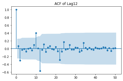
seasonal_lag = 12
display(stationarity_adf_test(raw.value.diff(seasonal_lag).dropna(), []))
display(stationarity_kpss_test(raw.value.diff(seasonal_lag).dropna(), []))
sm.graphics.tsa.plot_acf(raw.value.diff(seasonal_lag).dropna(), lags=50,
use_vlines=True, title='ACF of Lag{}'.format(seasonal_lag))
plt.tight_layout()
plt.show()
| Stationarity_adf | |
|---|---|
| Test Statistics | -4.30 |
| p-value | 0.00 |
| Used Lag | 11.00 |
| Used Observations | 54.00 |
| Critical Value(1%) | -3.56 |
| Maximum Information Criteria | 786.67 |
| Stationarity_kpss | |
|---|---|
| Test Statistics | 0.35 |
| p-value | 0.10 |
| Used Lag | 11.00 |
| Critical Value(10%) | 0.35 |
| Stationarity_adf | |
|---|---|
| Test Statistics | -2.14 |
| p-value | 0.23 |
| Used Lag | 11.00 |
| Used Observations | 48.00 |
| Critical Value(1%) | -3.57 |
| Maximum Information Criteria | 703.72 |
| Stationarity_kpss | |
|---|---|
| Test Statistics | 0.09 |
| p-value | 0.10 |
| Used Lag | 11.00 |
| Critical Value(10%) | 0.35 |
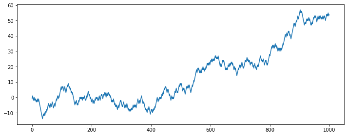
실습: 랜덤워크의 정상성 변환
# 라이브러리 호출
import pandas as pd
import numpy as np
import statsmodels.api as sm
from random import seed, random
import matplotlib.pyplot as plt
%reload_ext autoreload
%autoreload 2
from module import stationarity_adf_test, stationarity_kpss_test
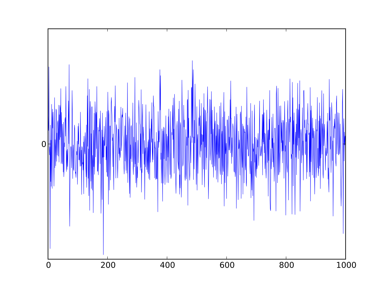
# 랜덤워크 데이터 생성
plt.figure(figsize=(10, 4))
seed(1)
random_walk = [-1 if random() < 0.5 else 1]
for i in range(1, 1000):
movement = -1 if random() < 0.5 else 1
value = random_walk[i-1] + movement
random_walk.append(value)
plt.plot(random_walk)
plt.tight_layout()
plt.show()
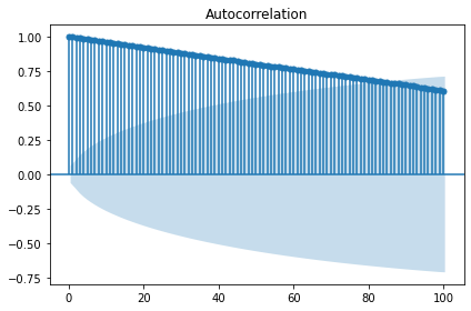
# 차분 전 랜덤워크 정상성 테스트
display('Before a difference:')
display(stationarity_adf_test(random_walk, []))
display(stationarity_kpss_test(random_walk, []))
sm.graphics.tsa.plot_acf(random_walk, lags=100, use_vlines=True)
plt.tight_layout()
plt.show()
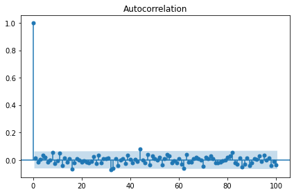
# 차분 후 랜덤워크 정상성 테스트
display('After a difference:')
display(stationarity_adf_test(pd.Series(random_walk).diff(1).dropna(), []))
display(stationarity_kpss_test(pd.Series(random_walk).diff(1).dropna(), []))
sm.graphics.tsa.plot_acf(pd.Series(random_walk).diff(1).dropna(), lags=100, use_vlines=True)
plt.tight_layout()
plt.show()
'Before a difference:'
| Stationarity_adf | |
|---|---|
| Test Statistics | 0.34 |
| p-value | 0.98 |
| Used Lag | 0.00 |
| Used Observations | 999.00 |
| Critical Value(1%) | -3.44 |
| Maximum Information Criteria | 2,773.39 |
| Stationarity_kpss | |
|---|---|
| Test Statistics | 3.75 |
| p-value | 0.01 |
| Used Lag | 22.00 |
| Critical Value(10%) | 0.35 |
'After a difference:'
| Stationarity_adf | |
|---|---|
| Test Statistics | -31.08 |
| p-value | 0.00 |
| Used Lag | 0.00 |
| Used Observations | 998.00 |
| Critical Value(1%) | -3.44 |
| Maximum Information Criteria | 2,770.18 |
| Stationarity_kpss | |
|---|---|
| Test Statistics | 0.22 |
| p-value | 0.10 |
| Used Lag | 22.00 |
| Critical Value(10%) | 0.35 |
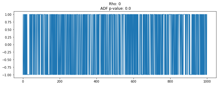
# 랜덤워크 데이터 생성 및 통계량 Test
plt.figure(figsize=(10, 4))
seed(1)
rho = 0
random_walk = [-1 if random() < 0.5 else 1]
for i in range(1, 1000):
    movement = -1 if random() < 0.5 else 1
    value = rho * random_walk[i-1] + movement
    random_walk.append(value)
plt.plot(random_walk)
plt.title('Rho: {}\n ADF p-value: {}'.format(rho, np.ravel(stationarity_adf_test(random_walk, []))[1]))
plt.tight_layout()
plt.show()

# rho 값을 변화시키면서 언제 비정상이 되는지 파악?
# 정상성의 계수 범위 추론 가능!
실습: 항공사 승객수요 스케일 변환(Log / Box-Cox)
# 라이브러리 호출
import numpy as np
import matplotlib.pyplot as plt
import statsmodels.api as sm
import scipy as sp
%reload_ext autoreload
%autoreload 2
from module import stationarity_adf_test, stationarity_kpss_test

# 데이터 준비
data = sm.datasets.get_rdataset("AirPassengers")
raw = data.data.copy()

# Box-Cox 변환 모수 추정
# 정규분포의 특정 범위(x)에서 lambda를 바꿔가며 정규성(measure:y)이 가장 높은 lambda(l_opt)를 선정
x, y = sp.stats.boxcox_normplot(raw.value, la=-3, lb=3)
y_transfer, l_opt = sp.stats.boxcox(raw.value)
print('Optimal Lambda: ', l_opt)

plt.plot(x, y)
plt.axvline(x=l_opt, color='r', ls="--")
plt.tight_layout()
plt.show()
Optimal Lambda: 0.14802265137037945
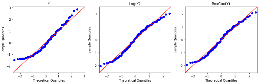
plt.figure(figsize=(12,4))
sm.qqplot(raw.value, fit=True, line='45', ax=plt.subplot(131))
plt.title('Y')
sm.qqplot(np.log(raw.value), fit=True, line='45', ax=plt.subplot(132))
plt.title('Log(Y)')
sm.qqplot(y_transfer, fit=True, line='45', ax=plt.subplot(133))
plt.title('BoxCox(Y)')
plt.tight_layout()
plt.show()
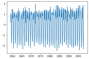
실습: 항공사 승객수요 정상성 변환
# 라이브러리 호출
import pandas as pd
import numpy as np
import matplotlib.pyplot as plt
import statsmodels.api as sm
%reload_ext autoreload
%autoreload 2
from module import stationarity_adf_test, stationarity_kpss_test
# 데이터 준비
data = sm.datasets.get_rdataset("AirPassengers")
raw = data.data.copy()
# 데이터 전처리
## 시간 인덱싱
if 'time' in raw.columns:
raw.index = pd.date_range(start='1/1/1949', periods=len(raw['time']), freq='M')
del raw['time']
## 정상성 확보
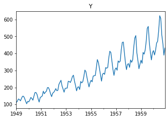
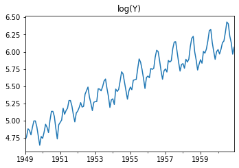
plt.figure(figsize=(12,8))
raw.plot(ax=plt.subplot(221), title='Y', legend=False)
np.log(raw).plot(ax=plt.subplot(222), title='log(Y)', legend=False)
raw.diff(1).plot(ax=plt.subplot(223), title='diff1(Y)', legend=False)
np.log(raw).diff(1).plot(ax=plt.subplot(224), title='diff1(log(Y))', legend=False)
plt.show()

## 정상성 테스트
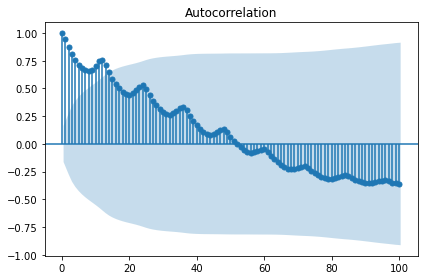
### 미변환
display('Non-transfer:')
plt.figure(figsize=(12,8))
raw.plot(ax=plt.subplot(222), title='Y', legend=False)
plt.show()
candidate_none = raw.copy()
display(stationarity_adf_test(candidate_none.values.flatten(), []))
display(stationarity_kpss_test(candidate_none.values.flatten(), []))
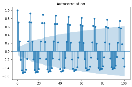
sm.graphics.tsa.plot_acf(candidate_none, lags=100, use_vlines=True)
plt.tight_layout()
plt.show()
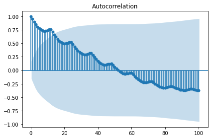
### 로그 변환
display('Log transfer:')
plt.figure(figsize=(12,8))
np.log(raw).plot(ax=plt.subplot(222), title='log(Y)', legend=False)
plt.show()
candidate_trend = np.log(raw).copy()
display(stationarity_adf_test(candidate_trend.values.flatten(), []))
display(stationarity_kpss_test(candidate_trend.values.flatten(), []))
sm.graphics.tsa.plot_acf(candidate_trend, lags=100, use_vlines=True)
plt.tight_layout()
plt.show()
trend_diff_order_initial = 0
result = stationarity_adf_test(candidate_trend.values.flatten(), []).T
if result['p-value'].values.flatten() < 0.1:
trend_diff_order = trend_diff_order_initial
else:
trend_diff_order = trend_diff_order_initial + 1
print('Trend Difference: ', trend_diff_order)
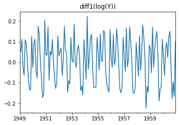
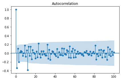
### 로그+추세차분 변환
display('Log and trend diffrence transfer:')
plt.figure(figsize=(12,8))
np.log(raw).diff(trend_diff_order).plot(ax=plt.subplot(224), title='diff1(log(Y))', legend=False)
plt.show()
candidate_seasonal = candidate_trend.diff(trend_diff_order).dropna().copy()
display(stationarity_adf_test(candidate_seasonal.values.flatten(), []))
display(stationarity_kpss_test(candidate_seasonal.values.flatten(), []))
sm.graphics.tsa.plot_acf(candidate_seasonal, lags=100, use_vlines=True)
plt.tight_layout()
plt.show()
seasonal_diff_order = sm.tsa.acf(candidate_seasonal)[1:].argmax() + 1
print('Seasonal Difference: ', seasonal_diff_order)
### 로그+추세차분+계절차분 변환
display('Log and trend+seasonal diffrence transfer:')
candidate_final = candidate_seasonal.diff(seasonal_diff_order).dropna().copy()
display(stationarity_adf_test(candidate_final.values.flatten(), []))
display(stationarity_kpss_test(candidate_final.values.flatten(), []))
sm.graphics.tsa.plot_acf(candidate_final, lags=100, use_vlines=True)
plt.tight_layout()
plt.show()
'Non-transfer:'
| Stationarity_adf | |
|---|---|
| Test Statistics | 0.82 |
| p-value | 0.99 |
| Used Lag | 13.00 |
| Used Observations | 130.00 |
| Critical Value(1%) | -3.48 |
| Maximum Information Criteria | 996.69 |
| Stationarity_kpss | |
|---|---|
| Test Statistics | 1.05 |
| p-value | 0.01 |
| Used Lag | 14.00 |
| Critical Value(10%) | 0.35 |
'Log transfer:'
| Stationarity_adf | |
|---|---|
| Test Statistics | -1.72 |
| p-value | 0.42 |
| Used Lag | 13.00 |
| Used Observations | 130.00 |
| Critical Value(1%) | -3.48 |
| Maximum Information Criteria | -445.40 |
| Stationarity_kpss | |
|---|---|
| Test Statistics | 1.05 |
| p-value | 0.01 |
| Used Lag | 14.00 |
| Critical Value(10%) | 0.35 |
Trend Difference: 1
'Log and trend diffrence transfer:'
| Stationarity_adf | |
|---|---|
| Test Statistics | -2.72 |
| p-value | 0.07 |
| Used Lag | 14.00 |
| Used Observations | 128.00 |
| Critical Value(1%) | -3.48 |
| Maximum Information Criteria | -440.36 |
| Stationarity_kpss | |
|---|---|
| Test Statistics | 0.10 |
| p-value | 0.10 |
| Used Lag | 14.00 |
| Critical Value(10%) | 0.35 |

Seasonal Difference: 12
'Log and trend+seasonal diffrence transfer:'
| Stationarity_adf | |
|---|---|
| Test Statistics | -4.44 |
| p-value | 0.00 |
| Used Lag | 12.00 |
| Used Observations | 118.00 |
| Critical Value(1%) | -3.49 |
| Maximum Information Criteria | -415.56 |
| Stationarity_kpss | |
|---|---|
| Test Statistics | 0.11 |
| p-value | 0.10 |
| Used Lag | 13.00 |
| Critical Value(10%) | 0.35 |
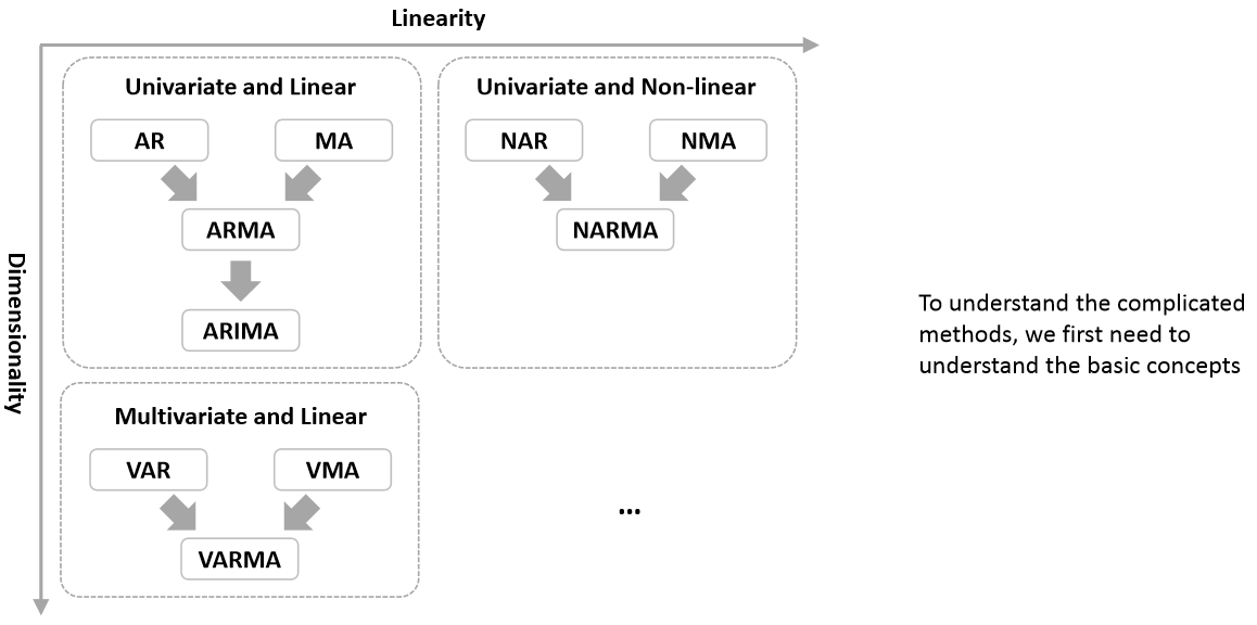
일반 선형확률과정(General Linear Process)
“시계열 데이터가 가우시안 백색잡음의 현재값과 과거값의 선형조합”
\begin{align*} Y_t = \epsilon_t + \psi_1\epsilon_{t-1} + \psi_2\epsilon_{t-2} + \cdots \ \end{align*} \begin{align*} where~\epsilon_i \sim i.i.d.~WN(0, \sigma_{\epsilon_i}^2)~and~\displaystyle \sum_{i=1}^{\infty}\psi_i^2 < \infty \end{align*}
세부 알고리즘:
WN(White Noise)
MA(Moving Average)
AR(Auto-Regressive)
ARMA(Auto-Regressive Moving Average)
ARIMA(Auto-Regressive Integrated Moving Average)
SARIMA(Seasonal ARIMA)
WN(White Noise)
1) 잔차들은 정규분포이고, (unbiased) 평균 0과 일정한 분산을 가져야 함:
\begin{align*} {\epsilon_t : t = \dots, -2, -1, 0, 1, 2, \dots} \sim N(0,\sigma^2_{\epsilon_t}) \ \end{align*} \begin{align*} where~~ \epsilon_t \sim i.i.d(independent~and~identically~distributed) \ \end{align*} \begin{align*} \epsilon_t = Y_t - \hat{Y_t}, ;; E(\epsilon_t) = 0, ;; Var(\epsilon_t) = \sigma^2_{\epsilon_t} \ \end{align*} \begin{align*} Cov(\epsilon_s, \epsilon_k) = 0~for~different~times!(s \ne k) \end{align*}
2) 잔차들이 시간의 흐름에 따라 상관성이 없어야 함:
자기상관함수(Autocorrelation Fundtion(ACF))를 통해 \(Autocorrelation~=~0\)인지 확인
공분산(Covariance):
$Cov(Y_s, Y_k)$ = $E[(Y_s-E(Y_s))$$(Y_k-E(Y_k))]$ = $\gamma_{s,k}$ - 자기상관함수(Autocorrelation Function):$Corr(Y_s, Y_k)$ = $\dfrac{Cov(Y_s, Y_k)}{\sqrt{Var(Y_s)Var(Y_k)}}$ = $\dfrac{\gamma_{s,k}}{\sqrt{\gamma_s \gamma_k}}$ - 편자기상관함수(Partial Autocorrelation Function): $s$와 $k$사이의 상관성을 제거한 자기상관함수$Corr[(Y_s-\hat{Y}_s, Y_{s-t}-\hat{Y}_{s-t})]$ for $1 특성요약:
강정상 과정(Stictly Stationary Process)
강정상 예시로 시계열분석 기본알고리즘 중 가장 중요함
시차(lag)가 0일 경우, 자기공분산은 확률 분포의 분산이 되고 시차가 0이 아닌 경우, 자기공분산은 0.
\begin{align*} \gamma_i = \begin{cases} \text{Var}(\epsilon_t) & ;; \text{ for } i = 0 \
0 & ;; \text{ for } i \neq 0 \end{cases} \end{align*}시차(lag)가 0일 경우, 자기상관계수는 1이 되고 시차가 0이 아닌 경우, 자기상관계수는 0. \begin{align*} \rho_i = \begin{cases} 1 & ;; \text{ for } i = 0 \
0 & ;; \text{ for } i \neq 0 \end{cases} \end{align*}
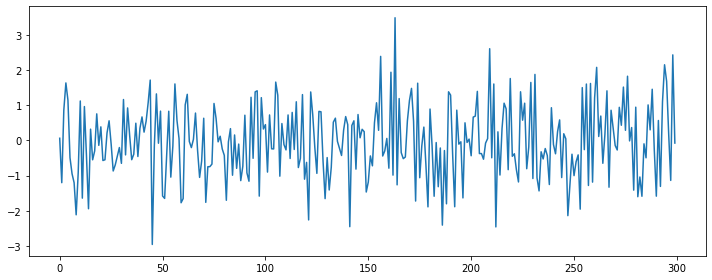
1) 예시: 가우시안 백색잡음
from scipy import stats
import matplotlib.pyplot as plt

plt.figure(figsize=(10, 4))
plt.plot(stats.norm.rvs(size=300))
plt.tight_layout()
plt.show()
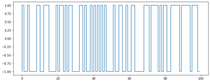
2) 예시: 베르누이 백색잡음
백색잡음의 기반 확률분포가 반드시 정규분포일 필요는 없음
import numpy as np
from scipy import stats
import matplotlib.pyplot as plt

plt.figure(figsize=(10, 4))
samples = stats.bernoulli.rvs(0.5, size=100) * 2 - 1
plt.step(np.arange(len(samples)), samples)
plt.ylim(-1.1, 1.1)
plt.tight_layout()
plt.show()
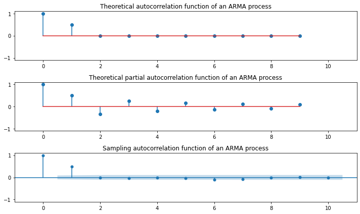
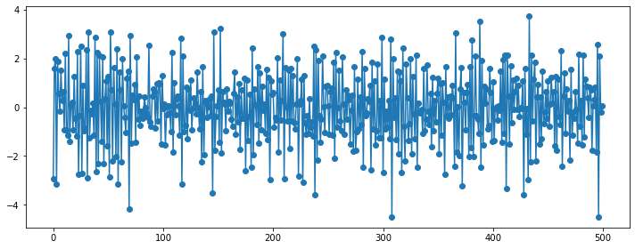
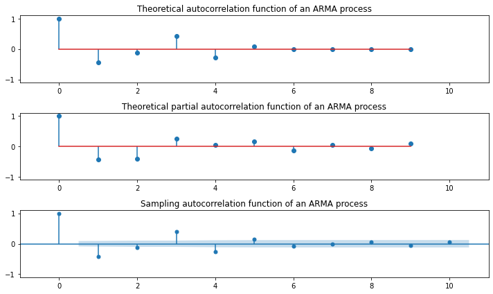
MA(Moving Average)
“\(MA(q)\): 알고리즘의 차수(\(q\))가 유한한 가우시안 백색잡음과정의 선형조합”
Exponential Smoothing 내 Moving Average Smoothing은 과거의 Trend-Cycle을 추정하기 위함이고, MA는 미래 값을 예측하기 위함
\begin{align*} Y_t &= \epsilon_t + \theta_1\epsilon_{t-1} + \theta_2\epsilon_{t-2} + \cdots + \theta_q\epsilon_{t-q} \end{align*} \begin{align*} where~\epsilon_i \sim i.i.d.~WN(0, \sigma_{\epsilon_i}^2)~and~\displaystyle \sum_{i=1}^{\infty}\theta_i^2 < \infty \end{align*} \begin{align*} Y_t &= \epsilon_t + \theta_1\epsilon_{t-1} + \theta_2\epsilon_{t-2} + \cdots + \theta_q\epsilon_{t-q} \ &= \epsilon_t + \theta_1L\epsilon_t + \theta_2L^2\epsilon_t + \cdots + \theta_qL^q\epsilon_t \ &= (1 + \theta_1L + \theta_2L^2 + \cdots + \theta_qL^q)\epsilon_t \ &= \theta(L)\epsilon_t \ \end{align*} \begin{align*} where~\epsilon_{t-1} = L\epsilon_t~and~\epsilon_{t-2} = L^2\epsilon_t$ \end{align*}
MA(1):
\begin{align*} \text{Main Equation} && Y_t &= \epsilon_t + \theta_1\epsilon_{t-1} \ \text{Expectation} && E(Y_t) &= E(\epsilon_t + \theta_1\epsilon_{t-1}) = E(\epsilon_t) + \theta_1E(\epsilon_{t-1}) = 0 \ \text{Variance} && Var(Y_t) &= E[(\epsilon_t + \theta_1\epsilon_{t-1})^2] \ && &= E(\epsilon_t^2) + 2\theta_1E(\epsilon_{t}\epsilon_{t-1}) + \theta_1^2E(\epsilon_{t-1}^2) \ && &= \sigma_{\epsilon_i}^2 + 2 \theta_1 \cdot 0 + \theta_1^2 \sigma_{\epsilon_i}^2 \ && &= \sigma_{\epsilon_i}^2 + \theta_1^2\sigma_{\epsilon_i}^2 \ \text{Covariance} && Cov(Y_t, Y_{t-1}) = \gamma_1 &= \text{E} \left[ (\epsilon_t + \theta_1 \epsilon_{t-1})(\epsilon_{t-1} + \theta_1 \epsilon_{t-2}) \right] \ && &= E (\epsilon_t \epsilon_{t-1}) + \theta_1 E (\epsilon_t \epsilon_{t-2}) + \theta_1 E (\epsilon_{t-1}^2) + \theta_1^2 E (\epsilon_{t-1} \epsilon_{t-2}) \ && &= 0 + \theta_1 \cdot 0 + \theta_1 \sigma_{\epsilon_{i}}^2 + \theta_1^2 \cdot 0 \ && &= \theta_1 \sigma_{\epsilon_{i}}^2 \ && Cov(Y_t, Y_{t-2}) = \gamma_2 &= \text{E} \left[ (\epsilon_t + \theta_1 \epsilon_{t-1})(\epsilon_{t-2} + \theta_1 \epsilon_{t-3}) \right] \ && &= E (\epsilon_t \epsilon_{t-2}) + \theta_1 E (\epsilon_t \epsilon_{t-3}) + \theta_1 E (\epsilon_{t-1} \epsilon_{t-2}) + \theta_1^2 E (\epsilon_{t-1} \epsilon_{t-3}) \ && &= 0 + \theta_1 \cdot 0 + \theta_1 \cdot 0 + \theta_1^2 \cdot 0 \ && &= 0 \ \text{Autocorrelation} && Corr(Y_t, Y_{t-1}) = \rho_1 &= \dfrac{\theta_1}{1+\theta_1^2} \ && Corr(Y_t, Y_{t-i}) = \rho_i &= 0~~for~~i > 1 \ \end{align*}MA(2):
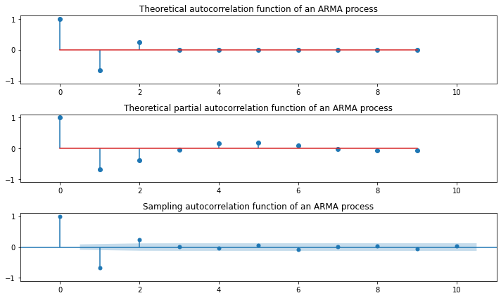
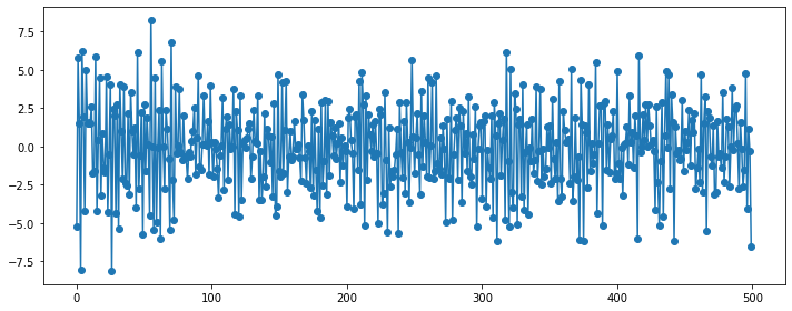
\begin{align*} \text{Main Equation} && Y_t &= \epsilon_t + \theta_1\epsilon_{t-1} + \theta_2\epsilon_{t-2} \ \text{Expectation} && E(Y_t) &= E(\epsilon_t + \theta_1\epsilon_{t-1} + \theta_2\epsilon_{t-2}) = E(\epsilon_t) + \theta_1E(\epsilon_{t-1}) + \theta_2E(\epsilon_{t-2}) = 0 \ \text{Variance} && Var(Y_t) &= E[(\epsilon_t + \theta_1\epsilon_{t-1} + \theta_2\epsilon_{t-2})^2] \ && &= \sigma_{\epsilon_i}^2 + \theta_1^2\sigma_{\epsilon_i}^2 + \theta_2^2\sigma_{\epsilon_i}^2 \ \text{Covariance} && Cov(Y_t, Y_{t-1}) = \gamma_1 &= \text{E} \left[ (\epsilon_t + \theta_1 \epsilon_{t-1} + \theta_2\epsilon_{t-2})(\epsilon_{t-1} + \theta_1 \epsilon_{t-2} + \theta_2\epsilon_{t-3}) \right] \ && &= (\theta_1 + \theta_1\theta_2) \sigma_{\epsilon_{i}}^2 \ && Cov(Y_t, Y_{t-2}) = \gamma_2 &= \text{E} \left[ (\epsilon_t + \theta_1 \epsilon_{t-1} + \theta_2\epsilon_{t-2})(\epsilon_{t-2} + \theta_1 \epsilon_{t-3} + \theta_2\epsilon_{t-4}) \right] \ && &= \theta_2 \sigma_{\epsilon_{i}}^2 \ && Cov(Y_t, Y_{t-i}) = \gamma_i &= 0~~for~~i > 2 \ \text{Autocorrelation} && Corr(Y_t, Y_{t-1}) = \rho_1 &= \dfrac{\theta_1 + \theta_1 \theta_2}{1+\theta_1^2+\theta_2^2} \ && Corr(Y_t, Y_{t-2}) = \rho_2 &= \dfrac{\theta_2}{1+\theta_1^2+\theta_2^2} \ && Corr(Y_t, Y_{t-i}) = \rho_i &= 0~~for~~i > 2 \ \end{align*}MA(q):
\begin{align*} \text{Autocorrelation} && Corr(Y_t, Y_{t-i}) = \rho_i &= \begin{cases} \dfrac{\theta_i + \theta_1\theta_{i-1} + \theta_2\theta_{i-2} + \cdots + \theta_q\theta_{i-q}}{1 + \theta_1^2 + \cdots + \theta_q^2} & \text{ for } i= 1, 2, \cdots, q \ 0 & \text{ for } i > q \ \end{cases} \end{align*}
움직임 특성:
Stationarity Condition of MA(1): \(|\theta_1| < 1\)
Stationarity Condition of MA(2): \(|\theta_2| < 1\), \(\theta_1 + \theta_2 > -1\), \(\theta_1 - \theta_2 < 1\)
import numpy as np
import statsmodels.api as sm
import matplotlib.pyplot as plt
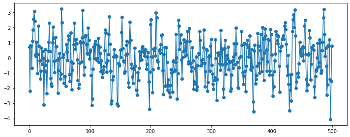
### MA(1)
plt.figure(figsize=(10, 4))
np.random.seed(123)
ar_params = np.array([])
ma_params = np.array([0.9])
ar, ma = np.r_[1, -ar_params], np.r_[1, ma_params]
y = sm.tsa.ArmaProcess(ar, ma).generate_sample(500, burnin=50)
plt.plot(y, 'o-')
plt.tight_layout()
plt.show()

plt.figure(figsize=(10, 6))
plt.subplot(311)
plt.stem(sm.tsa.ArmaProcess(ar, ma).acf(lags=10))
plt.xlim(-1, 11)
plt.ylim(-1.1, 1.1)
plt.title("Theoretical autocorrelation function of an ARMA process")

plt.subplot(312)
plt.stem(sm.tsa.ArmaProcess(ar, ma).pacf(lags=10))
plt.xlim(-1, 11)
plt.ylim(-1.1, 1.1)
plt.title("Theoretical partial autocorrelation function of an ARMA process")

sm.graphics.tsa.plot_acf(y, lags=10, ax=plt.subplot(313))
plt.xlim(-1, 11)
plt.ylim(-1.1, 1.1)
plt.title("Sampling autocorrelation function of an ARMA process")
plt.tight_layout()
plt.show()
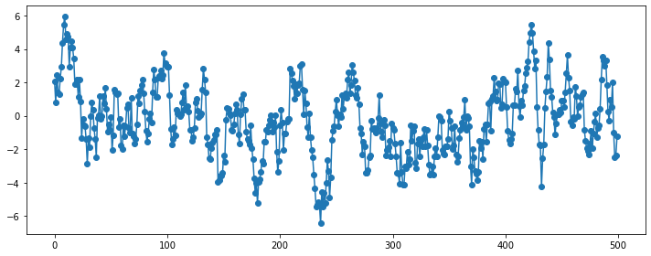
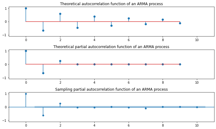
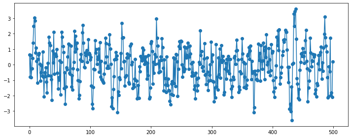
### MA(2)
plt.figure(figsize=(10, 4))
np.random.seed(123)
ar_params = np.array([])
ma_params = np.array([-1, 0.6])
ar, ma = np.r_[1, -ar_params], np.r_[1, ma_params]
y = sm.tsa.ArmaProcess(ar, ma).generate_sample(500, burnin=50)
plt.plot(y, 'o-')
plt.tight_layout()
plt.show()

plt.figure(figsize=(10, 6))
plt.subplot(311)
plt.stem(sm.tsa.ArmaProcess(ar, ma).acf(lags=10))
plt.xlim(-1, 11)
plt.ylim(-1.1, 1.1)
plt.title("Theoretical autocorrelation function of an ARMA process")

plt.subplot(312)
plt.stem(sm.tsa.ArmaProcess(ar, ma).pacf(lags=10))
plt.xlim(-1, 11)
plt.ylim(-1.1, 1.1)
plt.title("Theoretical partial autocorrelation function of an ARMA process")

sm.graphics.tsa.plot_acf(y, lags=10, ax=plt.subplot(313))
plt.xlim(-1, 11)
plt.ylim(-1.1, 1.1)
plt.title("Sampling autocorrelation function of an ARMA process")
plt.tight_layout()
plt.show()
### MA(5)
plt.figure(figsize=(10, 4))
np.random.seed(123)
ar_params = np.array([])
ma_params = np.array([-1, 1.6, 0.9, -1.5, 0.7])
ar, ma = np.r_[1, -ar_params], np.r_[1, ma_params]
y = sm.tsa.ArmaProcess(ar, ma).generate_sample(500, burnin=50)
plt.plot(y, 'o-')
plt.tight_layout()
plt.show()

plt.figure(figsize=(10, 6))
plt.subplot(311)
plt.stem(sm.tsa.ArmaProcess(ar, ma).acf(lags=10))
plt.xlim(-1, 11)
plt.ylim(-1.1, 1.1)
plt.title("Theoretical autocorrelation function of an ARMA process")

plt.subplot(312)
plt.stem(sm.tsa.ArmaProcess(ar, ma).pacf(lags=10))
plt.xlim(-1, 11)
plt.ylim(-1.1, 1.1)
plt.title("Theoretical partial autocorrelation function of an ARMA process")

sm.graphics.tsa.plot_acf(y, lags=10, ax=plt.subplot(313))
plt.xlim(-1, 11)
plt.ylim(-1.1, 1.1)
plt.title("Sampling autocorrelation function of an ARMA process")
plt.tight_layout()
plt.show()
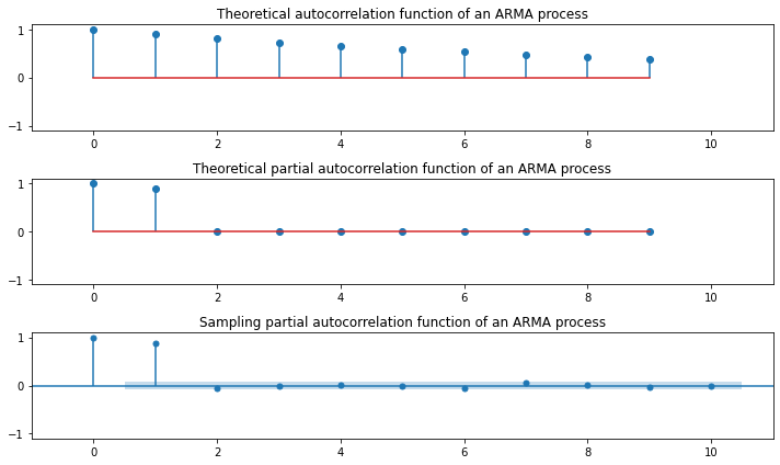
AR(Auto-Regressive)
“\(AR(p)\): 알고리즘의 차수(\(p\))가 유한한 자기자신의 과거값들의 선형조합”
필요성: ACF가 시차(Lag)가 증가해도 0이 되지 않고 오랜시간 남아있는 경우에 \(MA\)모형을 사용하면 차수가 \(\infty\)로 감
\begin{align*} Y_t &= \phi_1Y_{t-1} + \phi_2Y_{t-2} + \cdots + \phi_pY_{t-p} + \epsilon_t \ \end{align*} \begin{align*} where~\epsilon_i \sim i.i.d.~WN(0, \sigma_{\epsilon_i}^2)~and~\displaystyle \sum_{i=1}^{\infty}\phi_i^2 < \infty \end{align*} \begin{align*} Y_t &= \phi_1Y_{t-1} + \phi_2Y_{t-2} + \cdots + \phi_pY_{t-p} + \epsilon_t \ Y_t - \phi_1Y_{t-1} - \phi_2Y_{t-2} - \cdots - \phi_pY_{t-p} &= \epsilon_t \ Y_t - \phi_1LY_t - \phi_2L^2Y_t - \cdots - \phi_pL^pY_t &= \epsilon_t \ (1 - \phi_1L - \phi_2L^2 - \cdots - \phi_pL^p)Y_t &= \epsilon_t \ \phi(L)Y_t &= \epsilon_t \ \end{align*} \begin{align*} where~Y_{t-1} = LY_t~and~Y_{t-2} = L^2Y_t \end{align*}
AR(1):
\begin{align*} \text{Main Equation} && Y_t &= \phi_1 Y_{t-1} + \epsilon_t \ && &= \phi_1 (\phi_1 Y_{t-2} + \epsilon_{t-1}) + \epsilon_t \ && &= \phi_1^2 Y_{t-2} + \phi_1 \epsilon_{t-1} + \epsilon_t \ && &= \phi_1^2 (\phi_1 Y_{t-3} + \epsilon_{t-2}) + \phi_1 \epsilon_{t-1} + \epsilon_t \ && &= \phi_1^3 Y_{t-3} + \phi_1^2 \epsilon_{t-2} + \phi_1 \epsilon_{t-1} + \epsilon_t \ && & \vdots \ && &= \epsilon_t + \phi_1 \epsilon_{t-1} +\phi_1^2 \epsilon_{t-2} + \phi_1^3 \epsilon_{t-3} + \cdots \ && &= MA(\infty) \ \text{Expectation} && E(Y_t) &= \mu = E(\phi_1 Y_{t-1} + \epsilon_t) = \phi_1 E(Y_{t-1}) + E(\epsilon_{t}) = \phi_1 \mu + 0 \ && (1-\phi_1)\mu &= 0 \ && \mu &= 0~~if~~\phi_1 \neq 1 \ \text{Variance} && Var(Y_t) &= \gamma_0 = E(Y_t^2) = E[(\phi_1 Y_{t-1} + \epsilon_t)^2] = E[ \phi_1^2 Y_{t-1}^2 + 2\phi_1 Y_{t-1} \epsilon_{t} + \epsilon_{t}^2] \ && &= \phi_1^2 E[ Y_{t-1}^2 ] + 2 \phi E[ Y_{t-1} \epsilon_{t} ] + E[ \epsilon_{t}^2 ] \ && &= \phi_1^2 \gamma_0 + 0 + \sigma_{\epsilon_i}^2 \ && (1-\phi_1^2)\gamma_0 &= \sigma_{\epsilon_i}^2 \ && \gamma_0 &= \dfrac{\sigma_{\epsilon_i}^2}{1-\phi_1^2}~~if~~\phi_1^2 \neq 1 \ \text{Covariance} && Cov(Y_t, Y_{t-1}) &= \gamma_1 = E [(\phi_1 Y_{t-1} + \epsilon_t)(\phi_1 Y_{t-2} + \epsilon_{t-1})] \ && &= \phi_1^2E (Y_{t-1} Y_{t-2}) + \phi_1 E (Y_{t-1} \epsilon_{t-1}) + \phi_1 E (\epsilon_{t} Y_{t-2}) + E (\epsilon_{t} \epsilon_{t-1}) \ && &= \phi_1^2\gamma_1 + \phi_1 \sigma_{\epsilon_{i}}^2 + \phi_1 \cdot 0 + 0 \ && (1 - \phi_1^2)\gamma_1 &= \phi_1 \sigma_{\epsilon_{i}}^2 \ && \gamma_1 &= \dfrac{\phi_1 \sigma_{\epsilon_{i}}^2}{1 - \phi_1^2} \ && Cov(Y_t, Y_{t-2}) &= \gamma_2 = E [(\phi_1 Y_{t-1} + \epsilon_t)(\phi_1 Y_{t-3} + \epsilon_{t-2})] \ && &= \phi_1^2E (Y_{t-1} Y_{t-3}) + \phi_1 E (Y_{t-1} \epsilon_{t-2}) + \phi_1 E (\epsilon_{t} Y_{t-3}) + E (\epsilon_{t} \epsilon_{t-2}) \ && &= \phi_1^2\gamma_2 + \phi_1 E[(\phi_1Y_{t-2}+\epsilon_{t-1})\epsilon_{t-2}] + \phi_1 \cdot 0 + 0 \ && &= \phi_1^2\gamma_2 + \phi_1^2 E(Y_{t-2}\epsilon_{t-2}) + \phi_1 E(\epsilon_{t-1}\epsilon_{t-2}) \ && &= \phi_1^2\gamma_2 + \phi_1^2 \sigma_{\epsilon_{i}}^2 + 0 \ && (1 - \phi_1^2)\gamma_2 &= \phi_1^2 \sigma_{\epsilon_{i}}^2 \ && \gamma_2 &= \dfrac{\phi_1^2 \sigma_{\epsilon_{i}}^2}{1 - \phi_1^2} \ \text{Autocorrelation} && Corr(Y_t, Y_{t-1}) = \rho_1 &= \phi_1 \ && Corr(Y_t, Y_{t-2}) = \rho_2 &= \phi_1^2 \ && Corr(Y_t, Y_{t-i}) = \rho_i &= \phi_1^i \ \end{align*}
움직임 특성:
\(\phi_1 = 0\): \(Y_t\)는 백색잡음
\(\phi_1 < 0\): 부호를 바꿔가면서(진동하면서) 지수적으로 감소
\(\phi_1 > 0\): 시차가 증가하면서 자기상관계수는 지수적으로 감소
\(\phi_1 = 1\): \(Y_t\)는 비정상성인 랜덤워크(Random Walk) \begin{align*} Y_t &= Y_{t-1} + \epsilon_t \ Var(Y_t) &= Var(Y_{t-1} + \epsilon_t) \ &= Var(Y_{t-1}) + Var(\epsilon_t) ;; (\text{independence}) \ Var(Y_t) &> Var(Y_{t-1}) \end{align*}
Stationarity Condition: \(|\phi_1| < 1\)
AR(2):
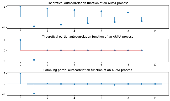
\begin{align*} \text{Main Equation} && Y_t &= \phi_1 Y_{t-1} + \phi_2 Y_{t-2} + \epsilon_t \ && &= \phi_1 (\phi_1 Y_{t-2} + \epsilon_{t-1}) + \phi_2 (\phi_2 Y_{t-3} + \epsilon_{t-2}) + \epsilon_t \ && &= \phi_1^2 Y_{t-2} + \phi_1 \epsilon_{t-1} + \phi_2^2 Y_{t-3} + \phi_2 \epsilon_{t-2} + \epsilon_t \ && &= \phi_1^2 (\phi_1 Y_{t-3} + \phi_2 Y_{t-4} + \epsilon_{t-3}) + \phi_1 \epsilon_{t-1} + \phi_2^2 (\phi_1 Y_{t-4} + \phi_2 Y_{t-5} + \epsilon_{t-4}) + \phi_2 \epsilon_{t-2} + \epsilon_t \ && & \vdots \ && &= \epsilon_t + \phi_1 \epsilon_{t-1} + \phi_2 \epsilon_{t-1} + \phi_1^2 \epsilon_{t-2} + \phi_2^2 \epsilon_{t-2} + \phi_1^3 \epsilon_{t-3} + \phi_2^3 \epsilon_{t-3} + \cdots \ && &= MA(\infty) \ \text{Expectation} && E(Y_t) &= \mu = E(\phi_1 Y_{t-1} + \phi_2 Y_{t-2} + \epsilon_t) = \phi_1 E(Y_{t-1}) + \phi_2 E(Y_{t-2}) + E(\epsilon_{t}) = \phi_1 \mu + \phi_2 \mu + 0 \ && (1-\phi_1-\phi_2)\mu &= 0 \ && \mu &= 0~~if~~\phi_1+\phi_2 \neq 1 \ \text{Covariance(“Yule-Walker Equation”)} && \gamma_i &= E(Y_tY_{t-i}) = E[(\phi_1 Y_{t-1} + \phi_2 Y_{t-2} + \epsilon_t)Y_{t-i}] \ && &= E(\phi_1 Y_{t-1}Y_{t-i}) + E(\phi_2 Y_{t-2}Y_{t-i}) + E(\epsilon_t Y_{t-i}) \ && &= \phi_1 \gamma_{i-1} + \phi_2 \gamma_{i-2} \ \text{Autocorrelation} && Corr(Y_t, Y_{t-i}) &= \rho_i = \phi_1 \rho_{i-1} + \phi_2 \rho_{i-2} \ && \rho_1 &= \phi_1 \rho_{0} + \phi_2 \rho_{-1} = \phi_1 \cdot 1 + \phi_2 \rho_{1} \ && (1-\phi_2)\rho_1 &= \phi_1 \ && \rho_1 &= \dfrac{\phi_1}{1-\phi_2} \ && & \vdots \ && \rho_2 &= \dfrac{\phi_1^2 + \phi_2(1-\phi_2)}{1-\phi_2} \ && & \vdots \ && \rho_i &= \left( 1+\dfrac{1+\phi_2}{1-\phi_2} \cdot i \right)\left(\dfrac{\phi_1}{2} \right)^i \ \end{align*}
움직임 특성:
시차가 증가하면서 자기상관계수의 절대값은 지수적으로 감소
진동 주파수에 따라 다르지만 진동 가능
Stationarity Condition: \(|\phi_1| < 1\), \(\phi_1 + \phi_2 < 1\), \(\phi_2 - \phi_1 < 1\)
import numpy as np
import statsmodels.api as sm
import matplotlib.pyplot as plt
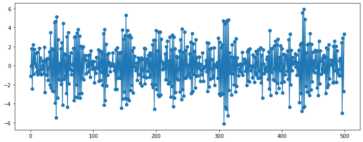
### AR(1)
plt.figure(figsize=(10, 4))
np.random.seed(123)
ar_params = np.array([0.9])
ma_params = np.array([])
ar, ma = np.r_[1, -ar_params], np.r_[1, ma_params]
y = sm.tsa.ArmaProcess(ar, ma).generate_sample(500, burnin=50)
plt.plot(y, 'o-')
plt.tight_layout()
plt.show()

plt.figure(figsize=(10, 6))
plt.subplot(311)
plt.stem(sm.tsa.ArmaProcess(ar, ma).acf(lags=10))
plt.xlim(-1, 11)
plt.ylim(-1.1, 1.1)
plt.title("Theoretical autocorrelation function of an ARMA process")

plt.subplot(312)
plt.stem(sm.tsa.ArmaProcess(ar, ma).pacf(lags=10))
plt.xlim(-1, 11)
plt.ylim(-1.1, 1.1)
plt.title("Theoretical partial autocorrelation function of an ARMA process")

sm.graphics.tsa.plot_pacf(y, lags=10, ax=plt.subplot(313))
plt.xlim(-1, 11)
plt.ylim(-1.1, 1.1)
plt.title("Sampling partial autocorrelation function of an ARMA process")
plt.tight_layout()
plt.show()
### AR(1)
plt.figure(figsize=(10, 4))
np.random.seed(123)
ar_params = np.array([-0.9])
ma_params = np.array([])
ar, ma = np.r_[1, -ar_params], np.r_[1, ma_params]
y = sm.tsa.ArmaProcess(ar, ma).generate_sample(500, burnin=50)
plt.plot(y, 'o-')
plt.tight_layout()
plt.show()

plt.figure(figsize=(10, 6))
plt.subplot(311)
plt.stem(sm.tsa.ArmaProcess(ar, ma).acf(lags=10))
plt.xlim(-1, 11)
plt.ylim(-1.1, 1.1)
plt.title("Theoretical autocorrelation function of an ARMA process")

plt.subplot(312)
plt.stem(sm.tsa.ArmaProcess(ar, ma).pacf(lags=10))
plt.xlim(-1, 11)
plt.ylim(-1.1, 1.1)
plt.title("Theoretical partial autocorrelation function of an ARMA process")

sm.graphics.tsa.plot_pacf(y, lags=10, ax=plt.subplot(313))
plt.xlim(-1, 11)
plt.ylim(-1.1, 1.1)
plt.title("Sampling partial autocorrelation function of an ARMA process")
plt.tight_layout()
plt.show()
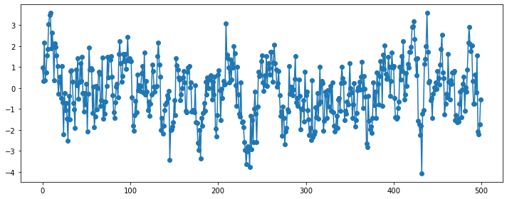
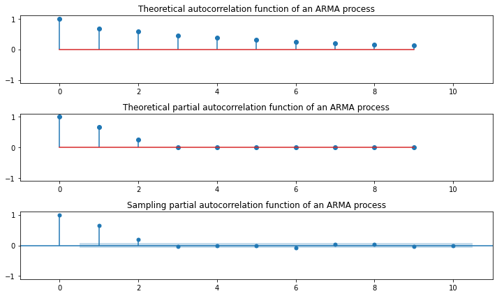
### AR(2)
plt.figure(figsize=(10, 4))
np.random.seed(123)
ar_params = np.array([0.5, 0.25])
ma_params = np.array([])
ar, ma = np.r_[1, -ar_params], np.r_[1, ma_params]
y = sm.tsa.ArmaProcess(ar, ma).generate_sample(500, burnin=50)
plt.plot(y, 'o-')
plt.tight_layout()
plt.show()

plt.figure(figsize=(10, 6))
plt.subplot(311)
plt.stem(sm.tsa.ArmaProcess(ar, ma).acf(lags=10))
plt.xlim(-1, 11)
plt.ylim(-1.1, 1.1)
plt.title("Theoretical autocorrelation function of an ARMA process")

plt.subplot(312)
plt.stem(sm.tsa.ArmaProcess(ar, ma).pacf(lags=10))
plt.xlim(-1, 11)
plt.ylim(-1.1, 1.1)
plt.title("Theoretical partial autocorrelation function of an ARMA process")

sm.graphics.tsa.plot_pacf(y, lags=10, ax=plt.subplot(313))
plt.xlim(-1, 11)
plt.ylim(-1.1, 1.1)
plt.title("Sampling partial autocorrelation function of an ARMA process")
plt.tight_layout()
plt.show()
### AR(2)
plt.figure(figsize=(10, 4))
np.random.seed(123)
ar_params = np.array([-0.5, 0.25])
ma_params = np.array([])
ar, ma = np.r_[1, -ar_params], np.r_[1, ma_params]
y = sm.tsa.ArmaProcess(ar, ma).generate_sample(500, burnin=50)
plt.plot(y, 'o-')
plt.tight_layout()
plt.show()

plt.figure(figsize=(10, 6))
plt.subplot(311)
plt.stem(sm.tsa.ArmaProcess(ar, ma).acf(lags=10))
plt.xlim(-1, 11)
plt.ylim(-1.1, 1.1)
plt.title("Theoretical autocorrelation function of an ARMA process")

plt.subplot(312)
plt.stem(sm.tsa.ArmaProcess(ar, ma).pacf(lags=10))
plt.xlim(-1, 11)
plt.ylim(-1.1, 1.1)
plt.title("Theoretical partial autocorrelation function of an ARMA process")

sm.graphics.tsa.plot_pacf(y, lags=10, ax=plt.subplot(313))
plt.xlim(-1, 11)
plt.ylim(-1.1, 1.1)
plt.title("Sampling partial autocorrelation function of an ARMA process")
plt.tight_layout()
plt.show()
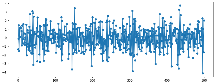
### AR(5)
plt.figure(figsize=(10, 4))
np.random.seed(123)
ar_params = np.array([0.5, 0.25, -0.3, 0.1, -0.1])
ma_params = np.array([])
ar, ma = np.r_[1, -ar_params], np.r_[1, ma_params]
y = sm.tsa.ArmaProcess(ar, ma).generate_sample(500, burnin=50)
plt.plot(y, 'o-')
plt.tight_layout()
plt.show()

plt.figure(figsize=(10, 6))
plt.subplot(311)
plt.stem(sm.tsa.ArmaProcess(ar, ma).acf(lags=10))
plt.xlim(-1, 11)
plt.ylim(-1.1, 1.1)
plt.title("Theoretical autocorrelation function of an ARMA process")

plt.subplot(312)
plt.stem(sm.tsa.ArmaProcess(ar, ma).pacf(lags=10))
plt.xlim(-1, 11)
plt.ylim(-1.1, 1.1)
plt.title("Theoretical partial autocorrelation function of an ARMA process")

sm.graphics.tsa.plot_pacf(y, lags=10, ax=plt.subplot(313))
plt.xlim(-1, 11)
plt.ylim(-1.1, 1.1)
plt.title("Sampling partial autocorrelation function of an ARMA process")
plt.tight_layout()
plt.show()
Relation of MA and AR
가역성 조건(Invertibility Condition):
1) \(MA(q)\) -> \(AR(\infty)\): 변환 후 AR 모형이 Stationary Condition이면 “Invertibility”
2) \(AR(p)\) -> \(MA(\infty)\): 여러개 모형변환 가능하지만 “Invertibility” 조건을 만족하는 MA 모형은 단 1개만 존재
ARMA(Auto-Regressive Moving Average)
“\(ARMA(p,q)\): 알고리즘의 차수(\(p~and~q\))가 유한한 \(AR(p)\)와 \(MA(q)\)의 선형조합”
\(AR\)과 \(MA\)의 정상성 조건과 가역성 조건이 동일하게 \(ARMA\) 알고리즘들에 적용
종속변수 \(Y_t\)는 종속변수 \(Y_t\)와 백색잡음(\(\epsilon_t\)) 차분들(Lagged Variables)의 합으로 예측가능
\begin{align*} Y_t = \phi_1Y_{t-1} + \phi_2Y_{t-2} + \cdots + \phi_pY_{t-p} + \theta_1\epsilon_{t-1} + \theta_2\epsilon_{t-2} + \cdots + \theta_q\epsilon_{t-q} + \epsilon_t \ \end{align*} \begin{align*} where~\epsilon_i \sim i.i.d.~WN(0, \sigma_{\epsilon_i}^2)~and~\displaystyle \sum_{i=1}^{\infty}\phi_i^2 < \infty, \displaystyle \sum_{i=1}^{\infty}\theta_i^2 < \infty \end{align*} \begin{align*} \phi(L)Y_t &= \theta(L)\epsilon_t \ Y_t &= \dfrac{\theta(L)}{\phi(L)}\epsilon_t \ \end{align*}
\begin{align*} \text{Main Equation} && Y_t &= \dfrac{\theta(L)}{\phi(L)}\epsilon_t \ && &= \psi(L)\epsilon_t \text{ where } \psi(L) = \dfrac{\theta(L)}{\phi(L)} \ && &= (1 + \psi_1L + \psi_2L^2 + \cdots)\epsilon_t \ && &= \epsilon_t + \psi_1\epsilon_{t-1} + \psi_2\epsilon_{t-2} + \cdots \ && & \text{ where } \ && \psi_1 &= \theta_1 - \phi_1 \ && \psi_2 &= \theta_2 - \phi_2 - \phi_1 \psi_1 \ && & \vdots \ && \psi_j &= \theta_j - \phi_p\psi_{j-p} - \phi_2 \psi_{p-1} - \cdots - \phi_1 \psi_{j-1} \ \text{Autocorrelation(“Yule-Walker Equation”)} && \rho_i &= \phi_1 \rho_{i-1} + \cdots + \phi_p \rho_{i-p} \ \end{align*}
import pandas as pd
import numpy as np
import statsmodels
import statsmodels.api as sm
import matplotlib.pyplot as plt
### ARMA(1,0) = AR(1)
# Setting
np.random.seed(123)
ar_params = np.array([0.75])
ma_params = np.array([])
index_name = ['const', 'ar(1)']
ahead = 100
ar, ma = np.r_[1, -ar_params], np.r_[1, ma_params]
ar_order, ma_order = len(ar)-1, len(ma)-1
# Generator
y = statsmodels.tsa.arima_process.arma_generate_sample(ar, ma, nsample=1000, burnin=500)
fit = statsmodels.tsa.arima_model.ARMA(y, (ar_order,ma_order)).fit(trend='c', disp=0)
pred_ts_point = fit.forecast(steps=ahead)[0]
pred_ts_interval = fit.forecast(steps=ahead)[2]
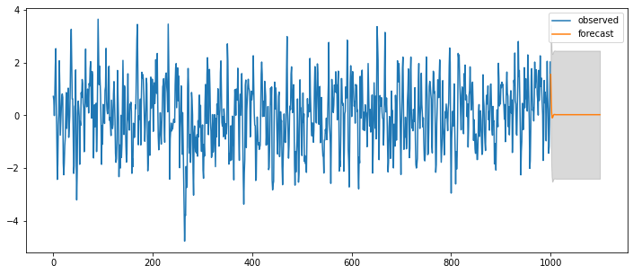
ax = pd.DataFrame(y).plot(figsize=(12,5))
forecast_index = [i for i in range(pd.DataFrame(y).index.max()+1, pd.DataFrame(y).index.max()+ahead+1)]
pd.DataFrame(pred_ts_point, index=forecast_index).plot(label='forecast', ax=ax)
ax.fill_between(pd.DataFrame(pred_ts_interval, index=forecast_index).index,
pd.DataFrame(pred_ts_interval, index=forecast_index).iloc[:,0],
pd.DataFrame(pred_ts_interval, index=forecast_index).iloc[:,1], color='k', alpha=0.15)
plt.legend(['observed', 'forecast'])
display(fit.summary2())
plt.figure(figsize=(12,3))
statsmodels.graphics.tsaplots.plot_acf(y, lags=50, zero=True, use_vlines=True, alpha=0.05, ax=plt.subplot(121))
statsmodels.graphics.tsaplots.plot_pacf(y, lags=50, zero=True, use_vlines=True, alpha=0.05, ax=plt.subplot(122))
plt.show()
| Model: | ARMA | BIC: | 2775.2536 |
| Dependent Variable: | y | Log-Likelihood: | -1377.3 |
| Date: | 2020-07-31 22:45 | Scale: | 1.0000 |
| No. Observations: | 1000 | Method: | css-mle |
| Df Model: | 2 | Sample: | 0 |
| Df Residuals: | 998 | 0 | |
| Converged: | 1.0000 | S.D. of innovations: | 0.959 |
| No. Iterations: | 4.0000 | HQIC: | 2766.126 |
| AIC: | 2760.5304 |
| Coef. | Std.Err. | t | P>|t| | [0.025 | 0.975] | |
|---|---|---|---|---|---|---|
| const | 0.0406 | 0.1197 | 0.3389 | 0.7347 | -0.1940 | 0.2752 |
| ar.L1.y | 0.7475 | 0.0210 | 35.6193 | 0.0000 | 0.7063 | 0.7886 |
| Real | Imaginary | Modulus | Frequency | |
|---|---|---|---|---|
| AR.1 | 1.3379 | 0.0000 | 1.3379 | 0.0000 |
### ARMA(2,0) = AR(2)
# Setting
np.random.seed(123)
ar_params = np.array([0.75, -0.25])
ma_params = np.array([])
index_name = ['const', 'ar(1)', 'ar(2)']
ahead = 100
ar, ma = np.r_[1, -ar_params], np.r_[1, ma_params]
ar_order, ma_order = len(ar)-1, len(ma)-1

# Generator
y = statsmodels.tsa.arima_process.arma_generate_sample(ar, ma, nsample=1000, burnin=500)
fit = statsmodels.tsa.arima_model.ARMA(y, (ar_order,ma_order)).fit(trend='c', disp=0)
pred_ts_point = fit.forecast(steps=ahead)[0]
pred_ts_interval = fit.forecast(steps=ahead)[2]
ax = pd.DataFrame(y).plot(figsize=(12,5))
forecast_index = [i for i in range(pd.DataFrame(y).index.max()+1, pd.DataFrame(y).index.max()+ahead+1)]
pd.DataFrame(pred_ts_point, index=forecast_index).plot(label='forecast', ax=ax)
ax.fill_between(pd.DataFrame(pred_ts_interval, index=forecast_index).index,
                pd.DataFrame(pred_ts_interval, index=forecast_index).iloc[:,0],
                pd.DataFrame(pred_ts_interval, index=forecast_index).iloc[:,1], color='k', alpha=0.15)
plt.legend(['observed', 'forecast'])
display(fit.summary2())
plt.figure(figsize=(12,3))
statsmodels.graphics.tsaplots.plot_acf(y, lags=50, zero=True, use_vlines=True, alpha=0.05, ax=plt.subplot(121))
statsmodels.graphics.tsaplots.plot_pacf(y, lags=50, zero=True, use_vlines=True, alpha=0.05, ax=plt.subplot(122))
plt.show()
| Model: | ARMA | BIC: | 2781.5944 |
| Dependent Variable: | y | Log-Likelihood: | -1377.0 |
| Date: | 2020-07-31 22:45 | Scale: | 1.0000 |
| No. Observations: | 1000 | Method: | css-mle |
| Df Model: | 3 | Sample: | 0 |
| Df Residuals: | 997 | 0 | |
| Converged: | 1.0000 | S.D. of innovations: | 0.959 |
| No. Iterations: | 5.0000 | HQIC: | 2769.424 |
| AIC: | 2761.9633 |
| Coef. | Std.Err. | t | P>|t| | [0.025 | 0.975] | |
|---|---|---|---|---|---|---|
| const | 0.0193 | 0.0592 | 0.3255 | 0.7448 | -0.0967 | 0.1352 |
| ar.L1.y | 0.7557 | 0.0305 | 24.7647 | 0.0000 | 0.6959 | 0.8155 |
| ar.L2.y | -0.2678 | 0.0305 | -8.7791 | 0.0000 | -0.3276 | -0.2080 |
| Real | Imaginary | Modulus | Frequency | |
|---|---|---|---|---|
| AR.1 | 1.4111 | -1.3203 | 1.9324 | -0.1197 |
| AR.2 | 1.4111 | 1.3203 | 1.9324 | 0.1197 |
### ARMA(4,0) = AR(4)
# Setting
np.random.seed(123)
ar_params = np.array([0.75, -0.25, 0.2, -0.5])
ma_params = np.array([])
index_name = ['const', 'ar(1)', 'ar(2)', 'ar(3)', 'ar(4)']
ahead = 100
ar, ma = np.r_[1, -ar_params], np.r_[1, ma_params]
ar_order, ma_order = len(ar)-1, len(ma)-1

# Generator
y = statsmodels.tsa.arima_process.arma_generate_sample(ar, ma, nsample=1000, burnin=500)
fit = statsmodels.tsa.arima_model.ARMA(y, (ar_order,ma_order)).fit(trend='c', disp=0)
pred_ts_point = fit.forecast(steps=ahead)[0]
pred_ts_interval = fit.forecast(steps=ahead)[2]
ax = pd.DataFrame(y).plot(figsize=(12,5))
forecast_index = [i for i in range(pd.DataFrame(y).index.max()+1, pd.DataFrame(y).index.max()+ahead+1)]
pd.DataFrame(pred_ts_point, index=forecast_index).plot(label='forecast', ax=ax)
ax.fill_between(pd.DataFrame(pred_ts_interval, index=forecast_index).index,
                pd.DataFrame(pred_ts_interval, index=forecast_index).iloc[:,0],
                pd.DataFrame(pred_ts_interval, index=forecast_index).iloc[:,1], color='k', alpha=0.15)
plt.legend(['observed', 'forecast'])
display(fit.summary2())
plt.figure(figsize=(12,3))
statsmodels.graphics.tsaplots.plot_acf(y, lags=50, zero=True, use_vlines=True, alpha=0.05, ax=plt.subplot(121))
statsmodels.graphics.tsaplots.plot_pacf(y, lags=50, zero=True, use_vlines=True, alpha=0.05, ax=plt.subplot(122))
plt.show()
| Model: | ARMA | BIC: | 2796.4388 |
| Dependent Variable: | y | Log-Likelihood: | -1377.5 |
| Date: | 2020-07-31 22:45 | Scale: | 1.0000 |
| No. Observations: | 1000 | Method: | css-mle |
| Df Model: | 5 | Sample: | 0 |
| Df Residuals: | 995 | 0 | |
| Converged: | 1.0000 | S.D. of innovations: | 0.958 |
| No. Iterations: | 12.0000 | HQIC: | 2778.184 |
| AIC: | 2766.9923 |
| Coef. | Std.Err. | t | P>|t| | [0.025 | 0.975] | |
|---|---|---|---|---|---|---|
| const | 0.0093 | 0.0374 | 0.2500 | 0.8026 | -0.0639 | 0.0826 |
| ar.L1.y | 0.7470 | 0.0279 | 26.7627 | 0.0000 | 0.6923 | 0.8017 |
| ar.L2.y | -0.2521 | 0.0362 | -6.9600 | 0.0000 | -0.3231 | -0.1811 |
| ar.L3.y | 0.1631 | 0.0362 | 4.4995 | 0.0000 | 0.0920 | 0.2341 |
| ar.L4.y | -0.4699 | 0.0279 | -16.8256 | 0.0000 | -0.5247 | -0.4152 |
| Real | Imaginary | Modulus | Frequency | |
|---|---|---|---|---|
| AR.1 | 0.8756 | -0.6261 | 1.0764 | -0.0988 |
| AR.2 | 0.8756 | 0.6261 | 1.0764 | 0.0988 |
| AR.3 | -0.7021 | -1.1592 | 1.3553 | -0.3367 |
| AR.4 | -0.7021 | 1.1592 | 1.3553 | 0.3367 |
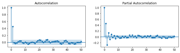
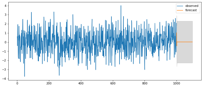
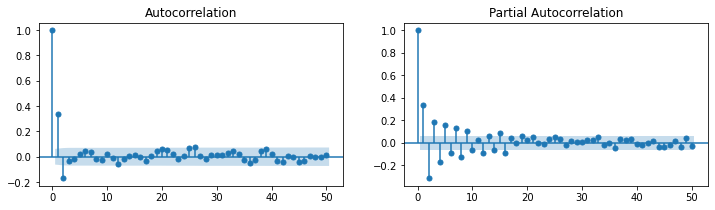
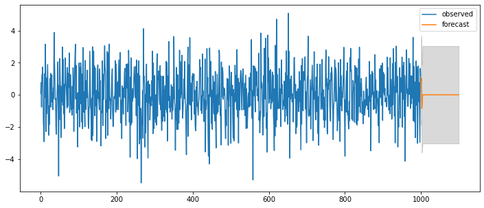
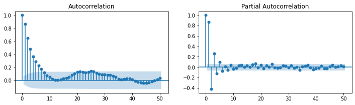
### ARMA(0,1) = MA(1)
# Setting
np.random.seed(123)
ar_params = np.array([])
ma_params = np.array([0.65])
index_name = ['const', 'ma(1)']
ahead = 100
ar, ma = np.r_[1, -ar_params], np.r_[1, ma_params]
ar_order, ma_order = len(ar)-1, len(ma)-1
# Generator
y = statsmodels.tsa.arima_process.arma_generate_sample(ar, ma, nsample=1000, burnin=500)
fit = statsmodels.tsa.arima_model.ARMA(y, (ar_order,ma_order)).fit(trend='c', disp=0)
pred_ts_point = fit.forecast(steps=ahead)[0]
pred_ts_interval = fit.forecast(steps=ahead)[2]
ax = pd.DataFrame(y).plot(figsize=(12,5))
forecast_index = [i for i in range(pd.DataFrame(y).index.max()+1, pd.DataFrame(y).index.max()+ahead+1)]
pd.DataFrame(pred_ts_point, index=forecast_index).plot(label='forecast', ax=ax)
ax.fill_between(pd.DataFrame(pred_ts_interval, index=forecast_index).index,
pd.DataFrame(pred_ts_interval, index=forecast_index).iloc[:,0],
pd.DataFrame(pred_ts_interval, index=forecast_index).iloc[:,1], color='k', alpha=0.15)
plt.legend(['observed', 'forecast'])
display(fit.summary2())
plt.figure(figsize=(12,3))
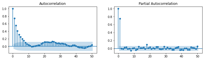
statsmodels.graphics.tsaplots.plot_acf(y, lags=50, zero=True, use_vlines=True, alpha=0.05, ax=plt.subplot(121))
statsmodels.graphics.tsaplots.plot_pacf(y, lags=50, zero=True, use_vlines=True, alpha=0.05, ax=plt.subplot(122))
plt.show()
| Model: | ARMA | BIC: | 2775.2511 |
| Dependent Variable: | y | Log-Likelihood: | -1377.3 |
| Date: | 2020-07-31 22:45 | Scale: | 1.0000 |
| No. Observations: | 1000 | Method: | css-mle |
| Df Model: | 2 | Sample: | 0 |
| Df Residuals: | 998 | 0 | |
| Converged: | 1.0000 | S.D. of innovations: | 0.959 |
| No. Iterations: | 3.0000 | HQIC: | 2766.124 |
| AIC: | 2760.5278 |
| Coef. | Std.Err. | t | P>|t| | [0.025 | 0.975] | |
|---|---|---|---|---|---|---|
| const | 0.0157 | 0.0500 | 0.3146 | 0.7531 | -0.0823 | 0.1138 |
| ma.L1.y | 0.6508 | 0.0246 | 26.5050 | 0.0000 | 0.6027 | 0.6989 |
| Real | Imaginary | Modulus | Frequency | |
|---|---|---|---|---|
| MA.1 | -1.5365 | 0.0000 | 1.5365 | 0.5000 |
### ARMA(0,2) = MA(2)
# Setting
np.random.seed(123)
ar_params = np.array([])
ma_params = np.array([0.65, -0.25])
index_name = ['const', 'ma(1)', 'ma(2)']
ahead = 100
ar, ma = np.r_[1, -ar_params], np.r_[1, ma_params]
ar_order, ma_order = len(ar)-1, len(ma)-1
# Generator
y = statsmodels.tsa.arima_process.arma_generate_sample(ar, ma, nsample=1000, burnin=500)
fit = statsmodels.tsa.arima_model.ARMA(y, (ar_order,ma_order)).fit(trend='c', disp=0)
pred_ts_point = fit.forecast(steps=ahead)[0]
pred_ts_interval = fit.forecast(steps=ahead)[2]
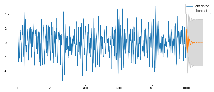
ax = pd.DataFrame(y).plot(figsize=(12,5))
forecast_index = [i for i in range(pd.DataFrame(y).index.max()+1, pd.DataFrame(y).index.max()+ahead+1)]
pd.DataFrame(pred_ts_point, index=forecast_index).plot(label='forecast', ax=ax)
ax.fill_between(pd.DataFrame(pred_ts_interval, index=forecast_index).index,
pd.DataFrame(pred_ts_interval, index=forecast_index).iloc[:,0],
pd.DataFrame(pred_ts_interval, index=forecast_index).iloc[:,1], color='k', alpha=0.15)
plt.legend(['observed', 'forecast'])
display(fit.summary2())
plt.figure(figsize=(12,3))
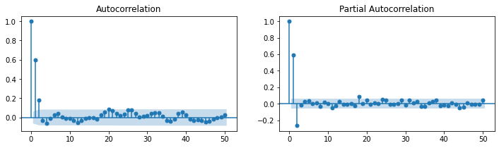
statsmodels.graphics.tsaplots.plot_acf(y, lags=50, zero=True, use_vlines=True, alpha=0.05, ax=plt.subplot(121))
statsmodels.graphics.tsaplots.plot_pacf(y, lags=50, zero=True, use_vlines=True, alpha=0.05, ax=plt.subplot(122))
plt.show()
| Model: | ARMA | BIC: | 2783.1398 |
| Dependent Variable: | y | Log-Likelihood: | -1377.8 |
| Date: | 2020-07-31 22:45 | Scale: | 1.0000 |
| No. Observations: | 1000 | Method: | css-mle |
| Df Model: | 3 | Sample: | 0 |
| Df Residuals: | 997 | 0 | |
| Converged: | 1.0000 | S.D. of innovations: | 0.959 |
| No. Iterations: | 8.0000 | HQIC: | 2770.970 |
| AIC: | 2763.5088 |
| Coef. | Std.Err. | t | P>|t| | [0.025 | 0.975] | |
|---|---|---|---|---|---|---|
| const | 0.0130 | 0.0425 | 0.3053 | 0.7602 | -0.0703 | 0.0962 |
| ma.L1.y | 0.6501 | 0.0310 | 20.9416 | 0.0000 | 0.5892 | 0.7109 |
| ma.L2.y | -0.2487 | 0.0307 | -8.0906 | 0.0000 | -0.3090 | -0.1885 |
| Real | Imaginary | Modulus | Frequency | |
|---|---|---|---|---|
| MA.1 | -1.0865 | 0.0000 | 1.0865 | 0.5000 |
| MA.2 | 3.7001 | 0.0000 | 3.7001 | 0.0000 |
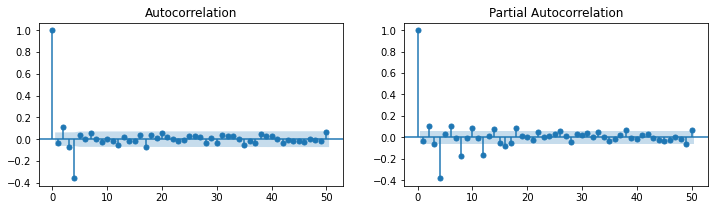
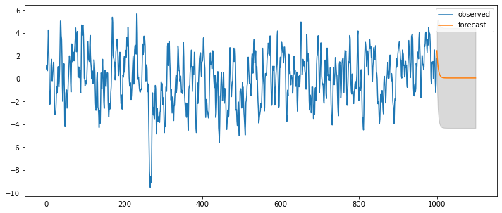
### ARMA(0,4) = MA(4)
# Setting
np.random.seed(123)
ar_params = np.array([])
ma_params = np.array([0.65, -0.25, 0.5, -0.9])
index_name = ['const', 'ma(1)', 'ma(2)', 'ma(3)', 'ma(4)']
ahead = 100
ar, ma = np.r_[1, -ar_params], np.r_[1, ma_params]
ar_order, ma_order = len(ar)-1, len(ma)-1

# Generator
y = statsmodels.tsa.arima_process.arma_generate_sample(ar, ma, nsample=1000, burnin=500)
fit = statsmodels.tsa.arima_model.ARMA(y, (ar_order,ma_order)).fit(trend='c', disp=0)
pred_ts_point = fit.forecast(steps=ahead)[0]
pred_ts_interval = fit.forecast(steps=ahead)[2]
ax = pd.DataFrame(y).plot(figsize=(12,5))
forecast_index = [i for i in range(pd.DataFrame(y).index.max()+1, pd.DataFrame(y).index.max()+ahead+1)]
pd.DataFrame(pred_ts_point, index=forecast_index).plot(label='forecast', ax=ax)
ax.fill_between(pd.DataFrame(pred_ts_interval, index=forecast_index).index,
                pd.DataFrame(pred_ts_interval, index=forecast_index).iloc[:,0],
                pd.DataFrame(pred_ts_interval, index=forecast_index).iloc[:,1], color='k', alpha=0.15)
plt.legend(['observed', 'forecast'])
display(fit.summary2())
plt.figure(figsize=(12,3))
statsmodels.graphics.tsaplots.plot_acf(y, lags=50, zero=True, use_vlines=True, alpha=0.05, ax=plt.subplot(121))
statsmodels.graphics.tsaplots.plot_pacf(y, lags=50, zero=True, use_vlines=True, alpha=0.05, ax=plt.subplot(122))
plt.show()
| Model: | ARMA | BIC: | 3472.2476 |
| Dependent Variable: | y | Log-Likelihood: | -1715.4 |
| Date: | 2020-07-31 22:45 | Scale: | 1.0000 |
| No. Observations: | 1000 | Method: | css-mle |
| Df Model: | 5 | Sample: | 0 |
| Df Residuals: | 995 | 0 | |
| Converged: | 1.0000 | S.D. of innovations: | 1.344 |
| No. Iterations: | 12.0000 | HQIC: | 3453.993 |
| AIC: | 3442.8011 |
| Coef. | Std.Err. | t | P>|t| | [0.025 | 0.975] | |
|---|---|---|---|---|---|---|
| const | 0.0079 | 0.0297 | 0.2653 | 0.7908 | -0.0504 | 0.0662 |
| ma.L1.y | -0.0418 | 0.0275 | -1.5186 | 0.1289 | -0.0957 | 0.0121 |
| ma.L2.y | 0.2823 | 0.0276 | 10.2186 | 0.0000 | 0.2282 | 0.3365 |
| ma.L3.y | -0.0569 | 0.0273 | -2.0805 | 0.0375 | -0.1105 | -0.0033 |
| ma.L4.y | -0.4858 | 0.0279 | -17.4311 | 0.0000 | -0.5404 | -0.4311 |
| Real | Imaginary | Modulus | Frequency | |
|---|---|---|---|---|
| MA.1 | 1.2761 | -0.0000 | 1.2761 | -0.0000 |
| MA.2 | -0.0088 | -1.0828 | 1.0829 | -0.2513 |
| MA.3 | -0.0088 | 1.0828 | 1.0829 | 0.2513 |
| MA.4 | -1.3757 | -0.0000 | 1.3757 | -0.5000 |
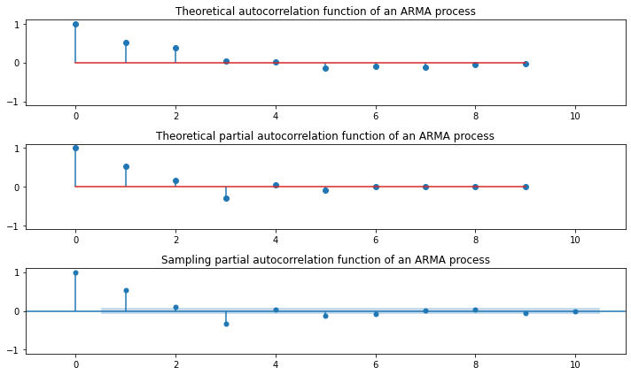
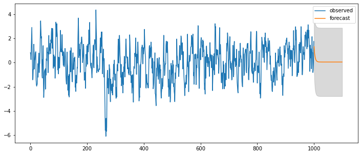
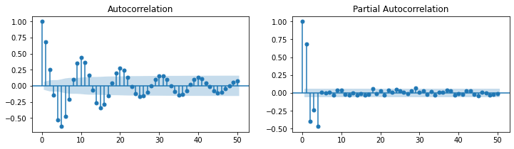
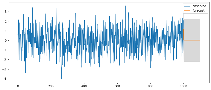
### ARMA(1,1)
# Setting
np.random.seed(123)
ar_params = np.array([0.75])
ma_params = np.array([0.65])
index_name = ['const', 'ar(1)', 'ma(1)']
ahead = 100
ar, ma = np.r_[1, -ar_params], np.r_[1, ma_params]
ar_order, ma_order = len(ar)-1, len(ma)-1

# Generator
y = statsmodels.tsa.arima_process.arma_generate_sample(ar, ma, nsample=1000, burnin=500)
fit = statsmodels.tsa.arima_model.ARMA(y, (ar_order,ma_order)).fit(trend='c', disp=0)
pred_ts_point = fit.forecast(steps=ahead)[0]
pred_ts_interval = fit.forecast(steps=ahead)[2]
ax = pd.DataFrame(y).plot(figsize=(12,5))
forecast_index = [i for i in range(pd.DataFrame(y).index.max()+1, pd.DataFrame(y).index.max()+ahead+1)]
pd.DataFrame(pred_ts_point, index=forecast_index).plot(label='forecast', ax=ax)
ax.fill_between(pd.DataFrame(pred_ts_interval, index=forecast_index).index,
                pd.DataFrame(pred_ts_interval, index=forecast_index).iloc[:,0],
                pd.DataFrame(pred_ts_interval, index=forecast_index).iloc[:,1], color='k', alpha=0.15)
plt.legend(['observed', 'forecast'])
display(fit.summary2())
plt.figure(figsize=(12,3))
statsmodels.graphics.tsaplots.plot_acf(y, lags=50, zero=True, use_vlines=True, alpha=0.05, ax=plt.subplot(121))
statsmodels.graphics.tsaplots.plot_pacf(y, lags=50, zero=True, use_vlines=True, alpha=0.05, ax=plt.subplot(122))
plt.show()
| Model: | ARMA | BIC: | 2783.7601 |
| Dependent Variable: | y | Log-Likelihood: | -1378.1 |
| Date: | 2020-07-31 22:45 | Scale: | 1.0000 |
| No. Observations: | 1000 | Method: | css-mle |
| Df Model: | 3 | Sample: | 0 |
| Df Residuals: | 997 | 0 | |
| Converged: | 1.0000 | S.D. of innovations: | 0.959 |
| No. Iterations: | 9.0000 | HQIC: | 2771.590 |
| AIC: | 2764.1291 |
| Coef. | Std.Err. | t | P>|t| | [0.025 | 0.975] | |
|---|---|---|---|---|---|---|
| const | 0.0641 | 0.1970 | 0.3252 | 0.7450 | -0.3220 | 0.4501 |
| ar.L1.y | 0.7465 | 0.0224 | 33.3502 | 0.0000 | 0.7027 | 0.7904 |
| ma.L1.y | 0.6519 | 0.0261 | 24.9637 | 0.0000 | 0.6007 | 0.7031 |
| Real | Imaginary | Modulus | Frequency | |
|---|---|---|---|---|
| AR.1 | 1.3395 | 0.0000 | 1.3395 | 0.0000 |
| MA.1 | -1.5340 | 0.0000 | 1.5340 | 0.5000 |
### ARMA(2,2)
# Setting
np.random.seed(123)
ar_params = np.array([0.75, -0.25])
ma_params = np.array([0.65, 0.5])
index_name = ['const', 'ar(1)', 'ar(2)', 'ma(1)', 'ma(2)']
ahead = 100
ar, ma = np.r_[1, -ar_params], np.r_[1, ma_params]
ar_order, ma_order = len(ar)-1, len(ma)-1

# Generator
y = statsmodels.tsa.arima_process.arma_generate_sample(ar, ma, nsample=1000, burnin=500)
fit = statsmodels.tsa.arima_model.ARMA(y, (ar_order,ma_order)).fit(trend='c', disp=0)
pred_ts_point = fit.forecast(steps=ahead)[0]
pred_ts_interval = fit.forecast(steps=ahead)[2]
ax = pd.DataFrame(y).plot(figsize=(12,5))
forecast_index = [i for i in range(pd.DataFrame(y).index.max()+1, pd.DataFrame(y).index.max()+ahead+1)]
pd.DataFrame(pred_ts_point, index=forecast_index).plot(label='forecast', ax=ax)
ax.fill_between(pd.DataFrame(pred_ts_interval, index=forecast_index).index,
                pd.DataFrame(pred_ts_interval, index=forecast_index).iloc[:,0],
                pd.DataFrame(pred_ts_interval, index=forecast_index).iloc[:,1], color='k', alpha=0.15)
plt.legend(['observed', 'forecast'])
display(fit.summary2())
plt.figure(figsize=(12,3))
statsmodels.graphics.tsaplots.plot_acf(y, lags=50, zero=True, use_vlines=True, alpha=0.05, ax=plt.subplot(121))
statsmodels.graphics.tsaplots.plot_pacf(y, lags=50, zero=True, use_vlines=True, alpha=0.05, ax=plt.subplot(122))
plt.show()
| Model: | ARMA | BIC: | 2796.4977 |
| Dependent Variable: | y | Log-Likelihood: | -1377.5 |
| Date: | 2020-07-31 22:45 | Scale: | 1.0000 |
| No. Observations: | 1000 | Method: | css-mle |
| Df Model: | 5 | Sample: | 0 |
| Df Residuals: | 995 | 0 | |
| Converged: | 1.0000 | S.D. of innovations: | 0.958 |
| No. Iterations: | 12.0000 | HQIC: | 2778.243 |
| AIC: | 2767.0512 |
| Coef. | Std.Err. | t | P>|t| | [0.025 | 0.975] | |
|---|---|---|---|---|---|---|
| const | 0.0415 | 0.1265 | 0.3283 | 0.7427 | -0.2065 | 0.2895 |
| ar.L1.y | 0.7472 | 0.0597 | 12.5090 | 0.0000 | 0.6301 | 0.8643 |
| ar.L2.y | -0.2675 | 0.0518 | -5.1626 | 0.0000 | -0.3691 | -0.1660 |
| ma.L1.y | 0.6544 | 0.0553 | 11.8393 | 0.0000 | 0.5460 | 0.7627 |
| ma.L2.y | 0.5209 | 0.0384 | 13.5542 | 0.0000 | 0.4456 | 0.5963 |
| Real | Imaginary | Modulus | Frequency | |
|---|---|---|---|---|
| AR.1 | 1.3966 | -1.3371 | 1.9334 | -0.1215 |
| AR.2 | 1.3966 | 1.3371 | 1.9334 | 0.1215 |
| MA.1 | -0.6281 | -1.2350 | 1.3855 | -0.3249 |
| MA.2 | -0.6281 | 1.2350 | 1.3855 | 0.3249 |
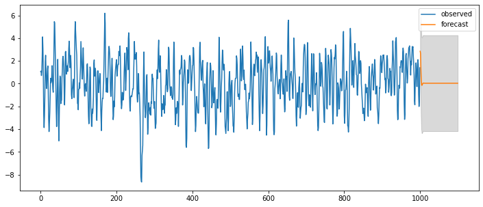
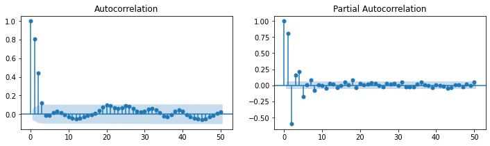
### ARMA(5,5)
# Setting
np.random.seed(123)
ar_params = np.array([0.75, -0.25, 0.5, -0.5, -0.1])
ma_params = np.array([0.65, 0.5, 0.2, -0.5, -0.1])
index_name = ['const', 'ar(1)', 'ar(2)', 'ar(3)', 'ar(4)', 'ar(5)', 'ma(1)', 'ma(2)', 'ma(3)', 'ma(4)', 'ma(5)']
ahead = 100
ar, ma = np.r_[1, -ar_params], np.r_[1, ma_params]
ar_order, ma_order = len(ar)-1, len(ma)-1

# Generator
y = statsmodels.tsa.arima_process.arma_generate_sample(ar, ma, nsample=1000, burnin=500)
fit = statsmodels.tsa.arima_model.ARMA(y, (ar_order,ma_order)).fit(trend='c', disp=0)
pred_ts_point = fit.forecast(steps=ahead)[0]
pred_ts_interval = fit.forecast(steps=ahead)[2]
ax = pd.DataFrame(y).plot(figsize=(12,5))
forecast_index = [i for i in range(pd.DataFrame(y).index.max()+1, pd.DataFrame(y).index.max()+ahead+1)]
pd.DataFrame(pred_ts_point, index=forecast_index).plot(label='forecast', ax=ax)
ax.fill_between(pd.DataFrame(pred_ts_interval, index=forecast_index).index,
                pd.DataFrame(pred_ts_interval, index=forecast_index).iloc[:,0],
                pd.DataFrame(pred_ts_interval, index=forecast_index).iloc[:,1], color='k', alpha=0.15)
plt.legend(['observed', 'forecast'])
display(fit.summary2())
plt.figure(figsize=(12,3))
statsmodels.graphics.tsaplots.plot_acf(y, lags=50, zero=True, use_vlines=True, alpha=0.05, ax=plt.subplot(121))
statsmodels.graphics.tsaplots.plot_pacf(y, lags=50, zero=True, use_vlines=True, alpha=0.05, ax=plt.subplot(122))
plt.show()

# ACF가 오히려 증가되는 이유는?
| Model: | ARMA | BIC: | 2844.4865 |
| Dependent Variable: | y | Log-Likelihood: | -1380.8 |
| Date: | 2020-07-31 22:46 | Scale: | 1.0000 |
| No. Observations: | 1000 | Method: | css-mle |
| Df Model: | 11 | Sample: | 0 |
| Df Residuals: | 989 | 0 | |
| Converged: | 1.0000 | S.D. of innovations: | 0.959 |
| No. Iterations: | 52.0000 | HQIC: | 2807.977 |
| AIC: | 2785.5934 |
| Coef. | Std.Err. | t | P>|t| | [0.025 | 0.975] | |
|---|---|---|---|---|---|---|
| const | 0.0308 | 0.0864 | 0.3569 | 0.7212 | -0.1386 | 0.2003 |
| ar.L1.y | 1.3387 | 0.4949 | 2.7049 | 0.0068 | 0.3687 | 2.3087 |
| ar.L2.y | -0.7833 | 0.4780 | -1.6387 | 0.1013 | -1.7202 | 0.1536 |
| ar.L3.y | 0.7138 | 0.2246 | 3.1786 | 0.0015 | 0.2737 | 1.1540 |
| ar.L4.y | -0.7758 | 0.2729 | -2.8428 | 0.0045 | -1.3106 | -0.2409 |
| ar.L5.y | 0.2339 | 0.2687 | 0.8705 | 0.3840 | -0.2927 | 0.7604 |
| ma.L1.y | 0.0678 | 0.4967 | 0.1365 | 0.8914 | -0.9057 | 1.0413 |
| ma.L2.y | 0.2093 | 0.2164 | 0.9674 | 0.3334 | -0.2148 | 0.6334 |
| ma.L3.y | -0.0514 | 0.1982 | -0.2592 | 0.7955 | -0.4398 | 0.3371 |
| ma.L4.y | -0.6159 | 0.0713 | -8.6360 | 0.0000 | -0.7557 | -0.4762 |
| ma.L5.y | 0.1658 | 0.2752 | 0.6027 | 0.5467 | -0.3735 | 0.7052 |
| Real | Imaginary | Modulus | Frequency | |
|---|---|---|---|---|
| AR.1 | -0.4994 | -1.1024 | 1.2103 | -0.3177 |
| AR.2 | -0.4994 | 1.1024 | 1.2103 | 0.3177 |
| AR.3 | 1.0036 | -0.5072 | 1.1245 | -0.0745 |
| AR.4 | 1.0036 | 0.5072 | 1.1245 | 0.0745 |
| AR.5 | 2.3086 | -0.0000 | 2.3086 | -0.0000 |
| MA.1 | -1.1194 | -0.0000 | 1.1194 | -0.5000 |
| MA.2 | -0.0971 | -1.0335 | 1.0381 | -0.2649 |
| MA.3 | -0.0971 | 1.0335 | 1.0381 | 0.2649 |
| MA.4 | 1.3648 | -0.0000 | 1.3648 | -0.0000 |
| MA.5 | 3.6627 | -0.0000 | 3.6627 | -0.0000 |
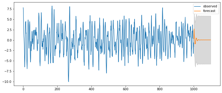
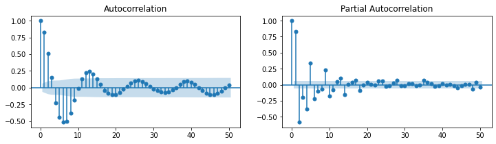
모형 차수결정 정리
1) 추정 및 예측을 하기 전에 파라미터에 따라 모형이 어떠한 결과를 도출할지 이해(예상) 필요
2) 결과이해(예상)는 기계의 실수를 방지하고 결과의 확신을 증가시킴
\(p\), \(q\) 파라미터 추론(by ACF and PACF):
정상성 형태 변환: 차분/로그변환/계절성제거 등을 통해 데이터를 정상성 형태로 변환
\(ACF\), \(PACF\)를 도식화 하여 ARMA의 파라미터 차수를 추론
- |
자기회귀: \(AR(p)\) |
이동평균: \(MA(q)\) |
자기회귀이동평균: \(ARMA(p,q)\) |
|---|---|---|---|
\(ACF\) |
지수적 감소, 진동하는 사인 형태 |
\(q+1\) 차항부터 절단모양(0수렴) |
\(q+1\) 차항부터 지수적 감소 혹은 진동하는 사인형태 |
\(PACF\) |
\(p+1\) 차항부터 절단모양(0수렴) |
지수적 감소, 진동하는 사인 형태 |
\(p+1\) 차항부터 지수적 감소 혹은 진동하는 사인형태 |
실습: 항체형성 호르몬수지 ARMA 모델링
import pandas as pd
import numpy as np
import matplotlib.pyplot as plt
import statsmodels.api as sm

# 데이터로딩 및 확인
data = sm.datasets.get_rdataset("lh")
raw = data.data
raw.plot(x='time', y='value')
plt.show()

# ACF/PACF 확인
plt.figure(figsize=(10, 8))
sm.graphics.tsa.plot_acf(raw.value, lags=10, ax=plt.subplot(211))
plt.xlim(-1, 11)
plt.ylim(-1.1, 1.1)
plt.title("ACF")

sm.graphics.tsa.plot_pacf(raw.value, lags=10, ax=plt.subplot(212))
plt.xlim(-1, 11)
plt.ylim(-1.1, 1.1)
plt.title("PACF")
plt.tight_layout()
plt.show()

# MA(1) 모델링
fit = sm.tsa.ARMA(raw.value, (0,1)).fit()
display(fit.summary())

# AR(1) 모델링
fit = sm.tsa.ARMA(raw.value, (1,0)).fit()
display(fit.summary())

# ARMA(1,1) 모델링
fit = sm.tsa.ARMA(raw.value, (1,1)).fit()
display(fit.summary())
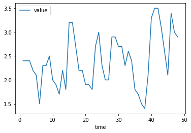
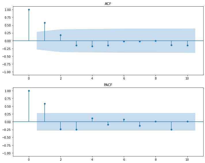
| Dep. Variable: | value | No. Observations: | 48 |
|---|---|---|---|
| Model: | ARMA(0, 1) | Log Likelihood | -31.052 |
| Method: | css-mle | S.D. of innovations | 0.461 |
| Date: | Fri, 31 Jul 2020 | AIC | 68.104 |
| Time: | 22:46:04 | BIC | 73.717 |
| Sample: | 0 | HQIC | 70.225 |
| coef | std err | z | P>|z| | [0.025 | 0.975] | |
|---|---|---|---|---|---|---|
| const | 2.4050 | 0.098 | 24.576 | 0.000 | 2.213 | 2.597 |
| ma.L1.value | 0.4810 | 0.094 | 5.093 | 0.000 | 0.296 | 0.666 |
| Real | Imaginary | Modulus | Frequency | |
|---|---|---|---|---|
| MA.1 | -2.0790 | +0.0000j | 2.0790 | 0.5000 |
| Dep. Variable: | value | No. Observations: | 48 |
|---|---|---|---|
| Model: | ARMA(1, 0) | Log Likelihood | -29.379 |
| Method: | css-mle | S.D. of innovations | 0.444 |
| Date: | Fri, 31 Jul 2020 | AIC | 64.758 |
| Time: | 22:46:04 | BIC | 70.372 |
| Sample: | 0 | HQIC | 66.880 |
| coef | std err | z | P>|z| | [0.025 | 0.975] | |
|---|---|---|---|---|---|---|
| const | 2.4133 | 0.147 | 16.460 | 0.000 | 2.126 | 2.701 |
| ar.L1.value | 0.5739 | 0.116 | 4.939 | 0.000 | 0.346 | 0.802 |
| Real | Imaginary | Modulus | Frequency | |
|---|---|---|---|---|
| AR.1 | 1.7424 | +0.0000j | 1.7424 | 0.0000 |
| Dep. Variable: | value | No. Observations: | 48 |
|---|---|---|---|
| Model: | ARMA(1, 1) | Log Likelihood | -28.762 |
| Method: | css-mle | S.D. of innovations | 0.439 |
| Date: | Fri, 31 Jul 2020 | AIC | 65.524 |
| Time: | 22:46:04 | BIC | 73.009 |
| Sample: | 0 | HQIC | 68.353 |
| coef | std err | z | P>|z| | [0.025 | 0.975] | |
|---|---|---|---|---|---|---|
| const | 2.4101 | 0.136 | 17.754 | 0.000 | 2.144 | 2.676 |
| ar.L1.value | 0.4522 | 0.177 | 2.556 | 0.011 | 0.105 | 0.799 |
| ma.L1.value | 0.1982 | 0.171 | 1.162 | 0.245 | -0.136 | 0.532 |
| Real | Imaginary | Modulus | Frequency | |
|---|---|---|---|---|
| AR.1 | 2.2114 | +0.0000j | 2.2114 | 0.0000 |
| MA.1 | -5.0462 | +0.0000j | 5.0462 | 0.5000 |
실습: 호흡기질환 사망자수 ARMA 모델링
import warnings
warnings.filterwarnings('always')
warnings.filterwarnings('ignore')

import pandas as pd
import numpy as np
import matplotlib.pyplot as plt
import statsmodels.api as sm

# 데이터로딩 및 확인
data = sm.datasets.get_rdataset("deaths", "MASS")
raw = data.data
raw.value = np.log(raw.value)
raw.plot(x='time', y='value')
plt.show()

# ACF/PACF 확인
plt.figure(figsize=(10, 8))
sm.graphics.tsa.plot_acf(raw.value.values, lags=50, ax=plt.subplot(211))
plt.xlim(-1, 51)
plt.ylim(-1.1, 1.1)
plt.title("ACF")

sm.graphics.tsa.plot_pacf(raw.value.values, lags=50, ax=plt.subplot(212))
plt.xlim(-1, 51)
plt.ylim(-1.1, 1.1)
plt.title("PACF")
plt.tight_layout()
plt.show()

# ARMA(1,1) 모델링
fit = sm.tsa.ARMA(raw.value, (1,1)).fit()
display(fit.summary())


| Dep. Variable: | value | No. Observations: | 72 |
|---|---|---|---|
| Model: | ARMA(1, 1) | Log Likelihood | 31.983 |
| Method: | css-mle | S.D. of innovations | 0.154 |
| Date: | Fri, 31 Jul 2020 | AIC | -55.965 |
| Time: | 22:46:06 | BIC | -46.859 |
| Sample: | 0 | HQIC | -52.340 |
| coef | std err | z | P>|z| | [0.025 | 0.975] | |
|---|---|---|---|---|---|---|
| const | 7.6037 | 0.080 | 94.470 | 0.000 | 7.446 | 7.761 |
| ar.L1.value | 0.6796 | 0.098 | 6.970 | 0.000 | 0.489 | 0.871 |
| ma.L1.value | 0.4680 | 0.111 | 4.214 | 0.000 | 0.250 | 0.686 |
| Real | Imaginary | Modulus | Frequency | |
|---|---|---|---|---|
| AR.1 | 1.4713 | +0.0000j | 1.4713 | 0.0000 |
| MA.1 | -2.1369 | +0.0000j | 2.1369 | 0.5000 |
from itertools import product

# ARMA(p,q) 모델링
result = []
for p, q in product(range(4), range(2)):
    if (p == 0 & q == 0):
        continue
    model = sm.tsa.ARMA(raw.value, (p, q)).fit()
    try:
        result.append({"p": p, "q": q, "LLF": model.llf, "AIC": model.aic, "BIC": model.bic})
    except:
        pass

# 모형 최적모수 선택
result = pd.DataFrame(result)
display(result)
opt_ar = result.iloc[np.argmin(result['AIC']), 0]
opt_ma = result.iloc[np.argmin(result['AIC']), 1]

# ARMA 모델링
fit = sm.tsa.ARMA(raw.value, (opt_ar,opt_ma)).fit()
display(fit.summary())

# 잔차 ACF/PACF 확인
plt.figure(figsize=(10, 8))
sm.graphics.tsa.plot_acf(fit.resid, lags=50, ax=plt.subplot(211))
plt.xlim(-1, 51)
plt.ylim(-1.1, 1.1)
plt.title("ACF")

sm.graphics.tsa.plot_pacf(fit.resid, lags=50, ax=plt.subplot(212))
plt.xlim(-1, 51)
plt.ylim(-1.1, 1.1)
plt.title("PACF")
plt.tight_layout()
plt.show()
| p | q | LLF | AIC | BIC | |
|---|---|---|---|---|---|
| 0 | 1 | 0 | 24.89 | -43.79 | -36.96 |
| 1 | 1 | 1 | 31.98 | -55.97 | -46.86 |
| 2 | 2 | 0 | 35.74 | -63.48 | -54.37 |
| 3 | 2 | 1 | 44.51 | -79.03 | -67.64 |
| 4 | 3 | 0 | 38.56 | -67.12 | -55.74 |
| 5 | 3 | 1 | 45.28 | -78.56 | -64.90 |
| Dep. Variable: | value | No. Observations: | 72 |
|---|---|---|---|
| Model: | ARMA(2, 1) | Log Likelihood | 44.513 |
| Method: | css-mle | S.D. of innovations | 0.128 |
| Date: | Fri, 31 Jul 2020 | AIC | -79.026 |
| Time: | 22:46:07 | BIC | -67.642 |
| Sample: | 0 | HQIC | -74.494 |
| coef | std err | z | P>|z| | [0.025 | 0.975] | |
|---|---|---|---|---|---|---|
| const | 7.5920 | 0.020 | 384.993 | 0.000 | 7.553 | 7.631 |
| ar.L1.value | 1.6407 | 0.059 | 27.830 | 0.000 | 1.525 | 1.756 |
| ar.L2.value | -0.8787 | 0.055 | -16.027 | 0.000 | -0.986 | -0.771 |
| ma.L1.value | -0.7021 | 0.075 | -9.363 | 0.000 | -0.849 | -0.555 |
| Real | Imaginary | Modulus | Frequency | |
|---|---|---|---|---|
| AR.1 | 0.9336 | -0.5162j | 1.0668 | -0.0804 |
| AR.2 | 0.9336 | +0.5162j | 1.0668 | 0.0804 |
| MA.1 | 1.4243 | +0.0000j | 1.4243 | 0.0000 |
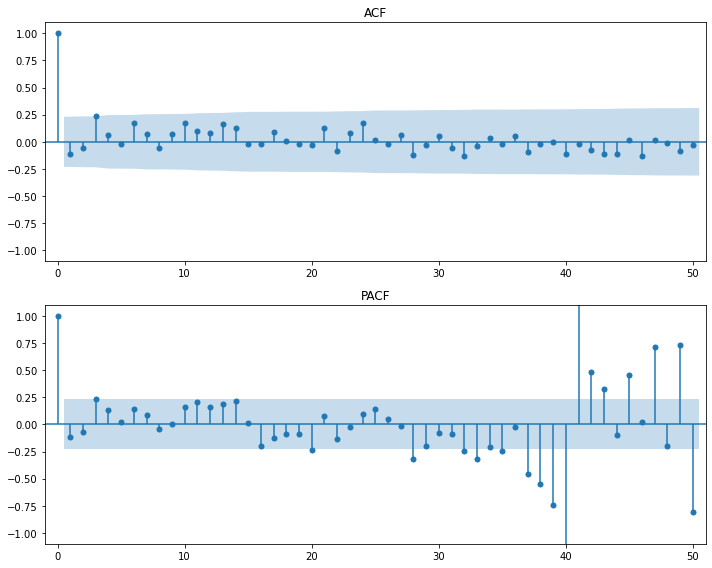
ARMAX(ARMA with eXogenous)
\begin{align*} \text{Equation of ARMA} && Y_t &= \phi_1Y_{t-1} + \phi_2Y_{t-2} + \cdots + \phi_pY_{t-p} + \theta_1\epsilon_{t-1} + \theta_2\epsilon_{t-2} + \cdots + \theta_q\epsilon_{t-q} + \epsilon_t \ \text{Equation of ARMAX} && Y_t &= \phi_1Y_{t-1} + \phi_2Y_{t-2} + \cdots + \phi_pY_{t-p} + \theta_1\epsilon_{t-1} + \theta_2\epsilon_{t-2} + \cdots + \theta_q\epsilon_{t-q} + \epsilon_t + \beta X \ \end{align*}
실습: 통화량을 고려한 소비자지출 ARMAX 모델링
import requests
from io import BytesIO
import pandas as pd
import numpy as np
import matplotlib.pyplot as plt
import statsmodels.api as sm

# 데이터 로딩 및 확인
source_url = requests.get('http://www.stata-press.com/data/r12/friedman2.dta').content
raw = pd.read_stata(BytesIO(source_url))
raw.index = raw.time
raw_using = raw.loc['1960':'1981',["consump", "m2"]]
raw_using.plot()
plt.show()

# 모델링
## 회귀분석
fit = sm.OLS(raw_using.consump, sm.add_constant(raw_using.m2)).fit()
display(fit.summary())

## 잔차 확인
fit.resid.plot()
plt.show()

## 잔차 ACF/PACF
plt.figure(figsize=(10, 8))
sm.graphics.tsa.plot_acf(fit.resid, lags=50, ax=plt.subplot(211))
plt.xlim(-1, 51)
plt.ylim(-1.1, 1.1)
plt.title("Residual ACF")

sm.graphics.tsa.plot_pacf(fit.resid, lags=50, ax=plt.subplot(212))
plt.xlim(-1, 51)
plt.ylim(-1.1, 1.1)
plt.title("Residual PACF")
plt.tight_layout()
plt.show()

# 모델링
## ARIMAX
fit = sm.tsa.ARMA(raw_using.consump, (1,1), exog=raw_using.m2).fit()
display(fit.summary())

## 잔차 확인
fit.resid.plot()
plt.show()

## 잔차 ACF/PACF
plt.figure(figsize=(10, 8))
sm.graphics.tsa.plot_acf(fit.resid, lags=50, ax=plt.subplot(211))
plt.xlim(-1, 51)
plt.ylim(-1.1, 1.1)
plt.title("Residual ACF")

sm.graphics.tsa.plot_pacf(fit.resid, lags=50, ax=plt.subplot(212))
plt.xlim(-1, 51)
plt.ylim(-1.1, 1.1)
plt.title("Residual PACF")
plt.tight_layout()
plt.show()
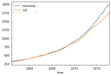
| Dep. Variable: | consump | R-squared: | 0.995 |
|---|---|---|---|
| Model: | OLS | Adj. R-squared: | 0.995 |
| Method: | Least Squares | F-statistic: | 1.721e+04 |
| Date: | Fri, 31 Jul 2020 | Prob (F-statistic): | 7.72e-101 |
| Time: | 22:46:10 | Log-Likelihood: | -434.48 |
| No. Observations: | 88 | AIC: | 873.0 |
| Df Residuals: | 86 | BIC: | 877.9 |
| Df Model: | 1 | ||
| Covariance Type: | nonrobust |
| coef | std err | t | P>|t| | [0.025 | 0.975] | |
|---|---|---|---|---|---|---|
| const | -61.7547 | 7.788 | -7.930 | 0.000 | -77.237 | -46.273 |
| m2 | 1.1406 | 0.009 | 131.182 | 0.000 | 1.123 | 1.158 |
| Omnibus: | 0.847 | Durbin-Watson: | 0.094 |
|---|---|---|---|
| Prob(Omnibus): | 0.655 | Jarque-Bera (JB): | 0.669 |
| Skew: | 0.213 | Prob(JB): | 0.716 |
| Kurtosis: | 2.984 | Cond. No. | 1.92e+03 |
Warnings:
[1] Standard Errors assume that the covariance matrix of the errors is correctly specified.
[2] The condition number is large, 1.92e+03. This might indicate that there are
strong multicollinearity or other numerical problems.
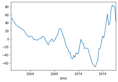
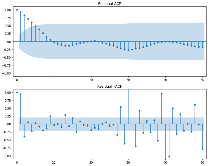
| Dep. Variable: | consump | No. Observations: | 88 |
|---|---|---|---|
| Model: | ARMA(1, 1) | Log Likelihood | -327.699 |
| Method: | css-mle | S.D. of innovations | 9.873 |
| Date: | Fri, 31 Jul 2020 | AIC | 665.398 |
| Time: | 22:46:11 | BIC | 677.784 |
| Sample: | 01-01-1960 | HQIC | 670.388 |
| - 10-01-1981 |
| coef | std err | z | P>|z| | [0.025 | 0.975] | |
|---|---|---|---|---|---|---|
| const | -37.6135 | 36.043 | -1.044 | 0.297 | -108.256 | 33.029 |
| m2 | 1.1232 | 0.034 | 33.282 | 0.000 | 1.057 | 1.189 |
| ar.L1.consump | 0.9330 | 0.043 | 21.867 | 0.000 | 0.849 | 1.017 |
| ma.L1.consump | 0.3106 | 0.116 | 2.682 | 0.007 | 0.084 | 0.538 |
| Real | Imaginary | Modulus | Frequency | |
|---|---|---|---|---|
| AR.1 | 1.0718 | +0.0000j | 1.0718 | 0.0000 |
| MA.1 | -3.2199 | +0.0000j | 3.2199 | 0.5000 |
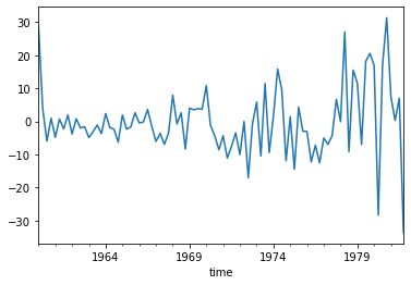
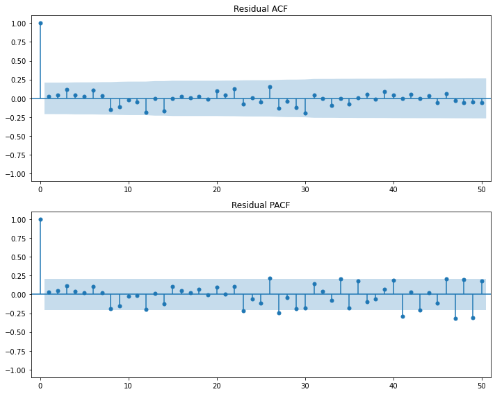
# 좀 더 적합성능을 높이는 방법은? ARMA의 한계는 추세차분!

# SARIMAX 모델링
fit = sm.tsa.SARIMAX(raw_using.consump, exog=raw_using.m2, order=(1,0,0), seasonal_order=(1,0,1,4)).fit()
display(fit.summary())

# 잔차 확인
fit.resid.plot()
plt.show()

# 잔차 ACF/PACF
plt.figure(figsize=(10, 8))
sm.graphics.tsa.plot_acf(fit.resid, lags=50, ax=plt.subplot(211))
plt.xlim(-1, 51)
plt.ylim(-1.1, 1.1)
plt.title("Residual ACF")

sm.graphics.tsa.plot_pacf(fit.resid, lags=50, ax=plt.subplot(212))
plt.xlim(-1, 51)
plt.ylim(-1.1, 1.1)
plt.title("Residual PACF")
plt.tight_layout()
plt.show()
| Dep. Variable: | consump | No. Observations: | 88 |
|---|---|---|---|
| Model: | SARIMAX(1, 0, 0)x(1, 0, [1], 4) | Log Likelihood | -333.579 |
| Date: | Fri, 31 Jul 2020 | AIC | 677.158 |
| Time: | 22:46:13 | BIC | 689.545 |
| Sample: | 01-01-1960 | HQIC | 682.148 |
| - 10-01-1981 | |||
| Covariance Type: | opg |
| coef | std err | z | P>|z| | [0.025 | 0.975] | |
|---|---|---|---|---|---|---|
| m2 | 0.3645 | 0.140 | 2.604 | 0.009 | 0.090 | 0.639 |
| ar.L1 | 0.9987 | 0.004 | 270.890 | 0.000 | 0.992 | 1.006 |
| ar.S.L4 | 0.9541 | 0.060 | 15.859 | 0.000 | 0.836 | 1.072 |
| ma.S.L4 | -0.4736 | 0.159 | -2.985 | 0.003 | -0.785 | -0.163 |
| sigma2 | 95.1802 | 9.448 | 10.074 | 0.000 | 76.662 | 113.699 |
| Ljung-Box (Q): | 47.49 | Jarque-Bera (JB): | 229.54 |
|---|---|---|---|
| Prob(Q): | 0.19 | Prob(JB): | 0.00 |
| Heteroskedasticity (H): | 23.47 | Skew: | -0.99 |
| Prob(H) (two-sided): | 0.00 | Kurtosis: | 10.66 |
Warnings:
[1] Covariance matrix calculated using the outer product of gradients (complex-step).
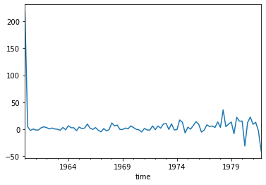
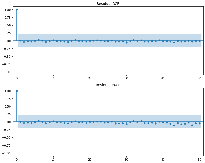
적분 선형확률과정(Integrated Linear Process)
ARIMA(Auto-Regressive Integrated Moving Average)
“\(ARIMA(p,d,q)\): 1이상의 차분이 적용된 \(\Delta^d Y_t = (1-L)^d Y_{t}\)가 알고리즘의 차수(\(p~and~q\))가 유한한 \(AR(p)\)와 \(MA(q)\)의 선형조합”
비정상성인 시계열 데이터 \(Y_t\)를 차분한 결과로 만들어진 \(\Delta Y_t = Y_t - Y_{t-1} = (1-L) Y_{t}\)가 정상성인 데이터이고 ARMA 모형을 따르면 원래의 \(Y_t\)를 ARIMA 모형이라고 함
=> \(d \geq 1\): \(Y_t\)는 비정상성 시계열 데이터이다(단위근을 갖는다)\(d\)번 차분한 후 시계열 \(\Delta^d Y_t\)가 정상성인 데이터이고 ARMA(p,q) 모형을 따른다면 적분차수(Order of Integrarion)가 \(d\)인 **ARIMA(p,d,q)**로 표기함
- \(p=0\): ARIMA(0,d,q) = IMA(d,q) - \(q=0\): ARIMA(p,d,0) = ARI(p,d)
Parameters |
Description |
|---|---|
\(p\) |
order of the autoregressive part |
\(d\) |
degree of differencing involved |
\(q\) |
order of the moving average part |
ARIMA(0,1,1) = IMA(1,1)
“자기상관계수(ACF)가 빠르게 감소하지 않는 것이 ARIMA와 같은 적분과정(Integrated Process)의 특징”
차분을 해야 정상성이 되는 \(Y_t\)이기에, 시차(Lag)가 증가해도 ACF가 1에 가까운 상관성을 유지하려 하기에 쉽게 감소하지 않음
\begin{align*} Y_t &= Y_{t-1} + \epsilon_t + \theta_1 \epsilon_{t-1} \ Y_t &= \epsilon_t+(1+\theta)\epsilon_{t-1}+(1+\theta)\epsilon_{t-2}+(1+\theta)\epsilon_{t-3}+\cdots \ Corr(Y_t, Y_{t-1}) &= \rho_i \approx 1 \end{align*}
ARIMA(0,2,1) = IMA(2,1)
\begin{align*} \Delta^2 Y_t = (1-L)^2 Y_{t} = \epsilon_t + \theta_1 \epsilon_{t-1}\ \end{align*}
ARIMA 모형 차수결정 정리
1) 추정 및 예측을 하기 전에 파라미터에 따라 모형이 어떠한 결과를 도출할지 이해(예상) 필요
2) 결과이해(예상)는 기계의 실수를 방지하고 결과의 확신을 증가시킴
\(p\), \(q\) 파라미터 추론(by ACF and PACF):
정상성 형태 변환: 차분/로그변환/계절성제거 등을 통해 데이터를 정상성 형태로 변환
\(ACF\), \(PACF\)를 도식화 하여 ARMA의 파라미터 차수를 추론
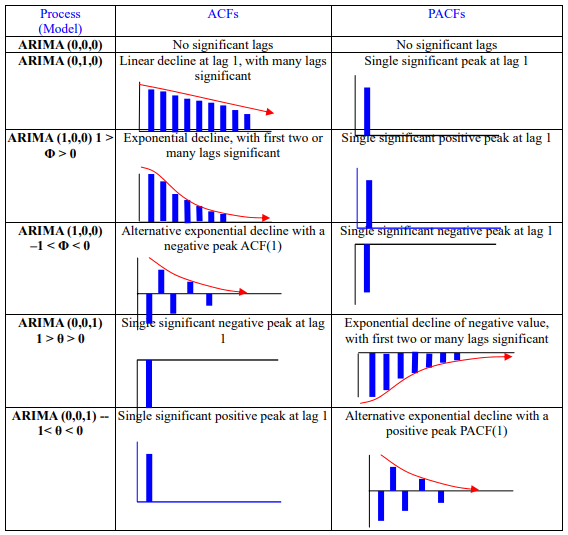
\(c\), \(d\) 파라미터 이해: X가 반영되지 않고 추정된 시계열 알고리즘은 결국 상수항의 적합성을 높이는 것!
“상수항(Const)인 \(c\)는 이론수식 복잡성으로 생략되기도 하나 존재가능”
“높은 차수의 차분(\(d\))은 예측 구간추정 범위를 급격하게 상승시킴”
\(c = 0, d = 0\): 점추정은 0, 예측의 구간추정은 과거데이터의 표준편차
\(c \neq 0, d = 0\): 점추정은 과거데이터의 평균, 예측의 구간추정은 과거데이터의 표준편차
\(p \geq 2\): 특정 변동(계절성, 싸이클)을 반영한 예측을 위해선 2이상의 차수 필수 - 예시: AR(2) 모형에서 \(\phi_1^2+4\phi_2<0\)를 만족해야 싸이클 형태로 예측되며 이때의 발생 싸이클은 다음과 같다 \begin{align*} \frac{2\pi}{\text{arc cos}(-\phi_1(1-\phi_2)/(4\phi_2))} \end{align*}
Parameters |
Long-term Forecasts |
|---|---|
\(c = 0, \\ d = 0\) |
go to zero |
\(c = 0, \\ d = 1\) |
go to a non-zero constant |
\(c = 0, \\ d = 2\) |
follow a straight line |
\(c \neq 0, \\ d = 0\) |
go to the mean of the data |
\(c \neq 0, \\ d = 1\) |
follow a straight line |
\(c \neq 0, \\ d = 2\) |
follow a quadratic trend |
import numpy as np
import statsmodels.api as sm
import matplotlib.pyplot as plt

# 2차누적/1차누적/미누적 데이터생성 및 적분차수 이해
np.random.seed(123)
y2 = sm.tsa.ArmaProcess([1], [1, 0.6]).generate_sample(100).cumsum().cumsum()
y1 = np.diff(y2)
y0 = np.diff(y1)

plt.figure(figsize=(10,8))
plt.subplot(311)
plt.title("ARIMA Simulation")
plt.plot(y2, 'o-')
plt.subplot(312)
plt.plot(y1, 'o-')
plt.subplot(313)
plt.plot(y0, 'o-')
plt.tight_layout()
plt.grid()
plt.show()
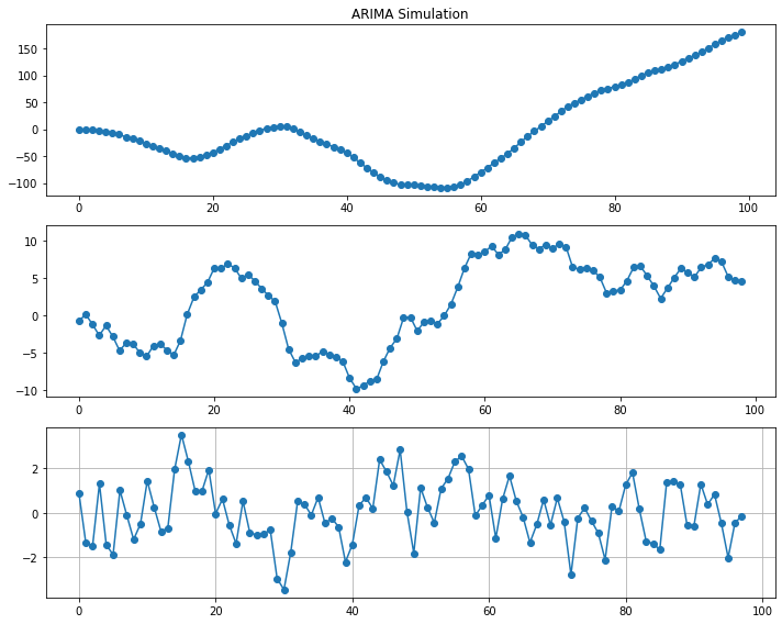
# 2차누적/1차누적/미누적 데이터시각화
plt.figure(figsize=(10,8))
sm.tsa.graphics.plot_acf(y2, ax=plt.subplot(311))
plt.grid()
sm.tsa.graphics.plot_acf(y1, ax=plt.subplot(312))
plt.grid()
sm.tsa.graphics.plot_acf(y0, ax=plt.subplot(313))
plt.grid()
plt.tight_layout()
plt.show()
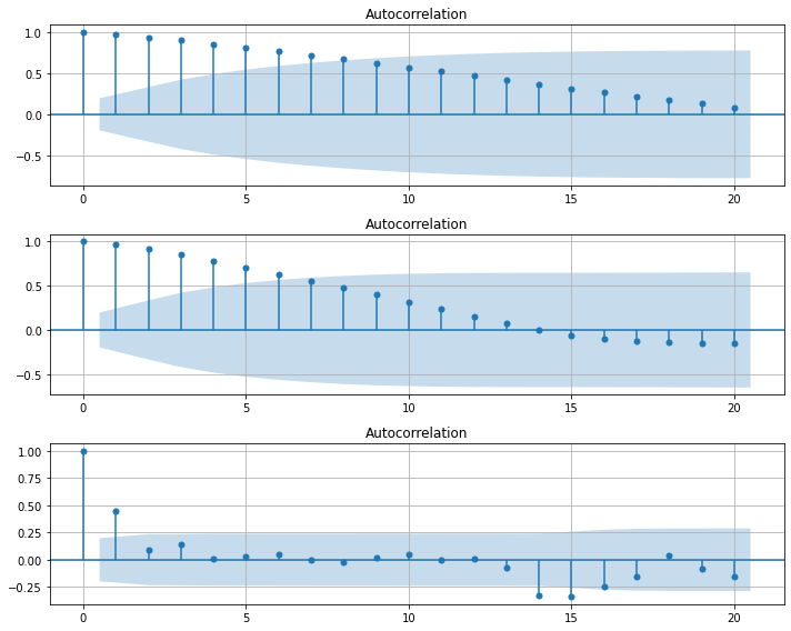
과차분(Over-differencing):
“필요 적분차수 이상의 차분은 MA모형을 생성!”
ARIMA(0,d,0) 모형을 따르는 \(Y_t\)를 \(d\)번 차분하면 백색잡음만 남음
추가 1차분: MA(1), 추가 2차분: MA(2)
과적합은 ACF/PACF의 수치를 오히려 증가시킬 수 있음
\begin{align*} \Delta^d Y_t &= \epsilon_t \ \Delta^{d+1} Y_t &= \epsilon_t - \epsilon_{t-1} \ \Delta^{d+2} Y_t &= \epsilon_t - 2\epsilon_{t-1} + \epsilon_{t-2} \ \end{align*}
# 과적차분 데이터 이해
y1_minus = np.diff(y0)

plt.figure(figsize=(10,8))
plt.subplot(211)
plt.plot(y1_minus, 'o-')
plt.title("Over-differencing 1 (Data)")
plt.grid()
sm.tsa.graphics.plot_acf(y1_minus, ax=plt.subplot(212))
plt.title("Over-differencing 1 (ACF)")
plt.grid()
plt.show()

y2_minus = np.diff(y1_minus)

plt.figure(figsize=(10,8))
plt.subplot(211)
plt.plot(y2_minus, 'o-')
plt.title("Over-differencing 2 (Data)")
plt.grid()
sm.tsa.graphics.plot_acf(y2_minus, ax=plt.subplot(212))
plt.title("Over-differencing 2 (ACF)")
plt.grid()
plt.show()
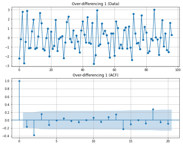
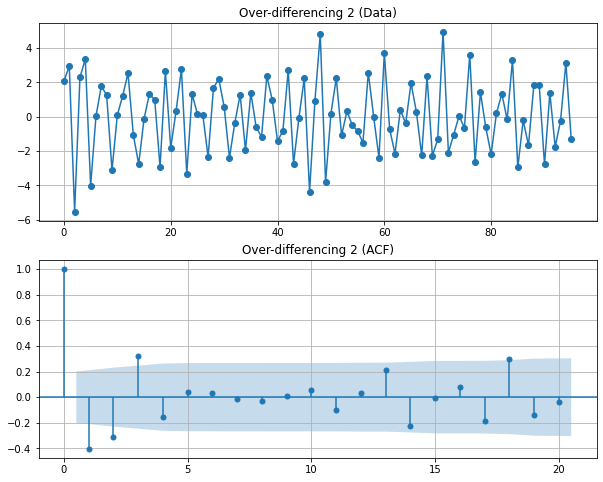
단위근 존재 의미:
“단위근을 갖는다는게 왜 비정상성 시계열 데이터라는 거지? -> \(d\) 차분을 해야 정상성이 되니까!”
“\(Y_t\)가 ARIMA(p,1,q)를 따른다” \(=\) “\(\Delta Y_t = Y_t - Y_{t-1}\)가 정상성이며 ARMA(p,q)를 따른다”
단위근이 있다는 것은 추세가 존재한다는 의미 -> 차분으로 추세제거 가능
\begin{align*} \text{Main Equation of ARIMA} && \Delta Y_t = \phi_1 \Delta Y_{t-1} + \phi_2 \Delta Y_{t-2} + \cdots + \phi_p \Delta Y_{t-p} + \theta_1 \epsilon_{t-1} + \theta_2 \epsilon_{t-2} + \cdots + \theta_q \epsilon_{t-q} + \epsilon_t \end{align*}
\begin{align*} \Delta Y_t - \phi_1 \Delta Y_{t-1} - \phi_2 \Delta Y_{t-2} - \cdots - \phi_p \Delta Y_{t-p} &= \theta_1 \epsilon_{t-1} + \theta_2 \epsilon_{t-2} + \cdots + \theta_q \epsilon_{t-q} + \epsilon_t \ Y_t-Y_{t-1} - \phi_1 (Y_{t-1}-Y_{t-2}) - \phi_2 (Y_{t-2}-Y_{t-3}) - \cdots - \phi_p (Y_{t-p}-Y_{t-p-1}) &= \epsilon_t + \theta_1 \epsilon_{t-1} + \theta_2 \epsilon_{t-2} + \cdots + \theta_q \epsilon_{t-q} \ Y_t - (\phi_1+1)Y_{t-1} - (\phi_2-\phi_1)Y_{t-2} - \cdots - (\phi_p-\phi_{p-1})Y_{t-p} + \phi_pY_{t-p-1} &= \epsilon_t+\theta_1\epsilon_{t-1}+\theta_2 \epsilon_{t-2}+\cdots+\theta_q \epsilon_{t-q} \ 1-(\phi_1+1)Y-(\phi_2-\phi_1)Y^2-\cdots-(\phi_p-\phi_{p-1})Y^p+\phi_pY^{p+1} &= 0 \ (1-Y)(1-\phi_1Y-\phi_2Y^2-\cdots-\phi_pY^p) &= 0 \ \end{align*}
\begin{align*} \text{Solution of ARIMA} && Y = 1 \text{ and } \sum_{i=1}^p \phi_i = 1 \end{align*}
\begin{align*} 1-\phi_1Y-\phi_2Y^2-\cdots-\phi_pY^p = 0 \ \end{align*}
\begin{align*} \text{Solution of ARMA} && \sum_{i=1}^p \phi_i = 1 \ \end{align*}
ARIMA 표현식 정리:
\begin{align*} \text{Main Equation of ARMA} && Y_t &= \phi_1Y_{t-1} + \phi_2Y_{t-2} + \cdots + \phi_pY_{t-p} + \theta_1\epsilon_{t-1} + \theta_2\epsilon_{t-2} + \cdots + \theta_q\epsilon_{t-q} + \epsilon_t \ && \phi(L)Y_t &= \theta(L)\epsilon_t \ \text{Main Equation of ARIMA} && (1-L)^d Y_t &= \phi_1 (1-L)^d Y_{t-1} + \phi_2 (1-L)^d Y_{t-2} + \cdots + \phi_p (1-L)^d Y_{t-p} + \theta_1\epsilon_{t-1} + \theta_2\epsilon_{t-2} + \cdots + \theta_q\epsilon_{t-q} + \epsilon_t \ && \phi(L)(1-L)^dY_t &= \theta(L)\epsilon_t \ \end{align*}
\begin{equation} \begin{array}{c c c c} (1-\phi_1L - \cdots - \phi_p L^p) & (1-L)^d Y_{t} &= (1 + \theta_1 L + \cdots + \theta_q L^q)\epsilon_t\ {\uparrow} & {\uparrow} & {\uparrow}\ \text{AR(\(p\))} & \text{\(d\) differences} & \text{MA(\(q\))}\ \end{array} \end{equation}
Time Series Algorithms |
ARIMA Expressions |
|---|---|
White noise |
ARIMA(0,0,0) |
Random walk |
ARIMA(0,1,0) |
Autoregression(\(AR(p)\)) |
ARIMA(\(p\),0,0) |
Moving average(\(MA(q)\)) |
ARIMA(0,0,\(q\)) |
\begin{align*} \text{Main Equation of ARIMA} && (1-\phi_1L - \cdots - \phi_p L^p) (1-L)^d Y_{t} &= (1 + \theta_1 L + \cdots + \theta_q L^q)\epsilon_t\ \text{Main Equation of ARIMAX} && (1-\phi_1L - \cdots - \phi_p L^p) (1-L)^d Y_{t} &= \sum^{k}{i=1}\beta{i}Z_{it} + (1 + \theta_1 L + \cdots + \theta_q L^q)\epsilon_t\ \end{align*}
import pandas as pd
import numpy as np
from statsmodels import datasets
import matplotlib.pyplot as plt
import statsmodels.api as sm
%reload_ext autoreload
%autoreload 2
from module import stationarity_adf_test, stationarity_kpss_test
# ARIMA 모형의 한계
# 데이터 로딩 및 시간변수 반영
raw_set = datasets.get_rdataset("accdeaths", package="MASS")
raw = raw_set.data
raw.time = pd.date_range('1973-01-01', periods=len(raw), freq='M')
raw['month'] = raw.time.dt.month

# 데이터 확인
display(raw.tail())
plt.plot(raw.time, raw.value)
plt.show()

# 정상성 확인
display(stationarity_adf_test(raw.value, []))
display(stationarity_kpss_test(raw.value, []))
sm.graphics.tsa.plot_acf(raw.value, lags=50, use_vlines=True)
plt.tight_layout()
plt.show()
| time | value | month | |
|---|---|---|---|
| 67 | 1978-08-31 | 9827 | 8 |
| 68 | 1978-09-30 | 9110 | 9 |
| 69 | 1978-10-31 | 9070 | 10 |
| 70 | 1978-11-30 | 8633 | 11 |
| 71 | 1978-12-31 | 9240 | 12 |
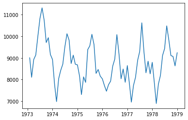
| Stationarity_adf | |
|---|---|
| Test Statistics | -2.54 |
| p-value | 0.11 |
| Used Lag | 12.00 |
| Used Observations | 59.00 |
| Critical Value(1%) | -3.55 |
| Maximum Information Criteria | 870.44 |
| Stationarity_kpss | |
|---|---|
| Test Statistics | 0.28 |
| p-value | 0.10 |
| Used Lag | 12.00 |
| Critical Value(10%) | 0.35 |
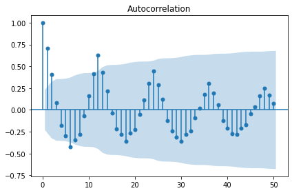
SARIMA(Seasonal ARIMA)
“ARIMA 모형은 Non-seasonal 데이터 또는 Non-seasonal ARIMA 모델을 가정 -> 계절성 패턴 반영 모델 필요!”
SARIMAX 클래스 이용하면 Multiplicated SARIMA(p,d,q)x(P,D,Q,m) 모형 추정 및 예측 가능
SARIMAX의 fit 메서드는 모수를 추정하여 그 결과를 SARIMAXResult 클래스 인스턴스로 반환
\begin{align*} \text{SARIMA} && \underbrace{(p, d, q)} && \underbrace{(P, D, Q)_m} \ && {\uparrow} && {\uparrow} \ && \text{Non-seasonal part} && \text{Seasonal part} \ && \text{of the model} && \text{of the model} \ \end{align*}
\begin{align*} \text{where } m = \text{ seasonal lag of observations.} \end{align*}
\begin{align*} \text{Equation: ARIMA(p,d,q)} && (1-\phi_1L - \cdots - \phi_p L^p) (1-L)^d Y_{t} &= (1 + \theta_1 L + \cdots + \theta_q L^q) \epsilon_t\ \text{Equation: ARIMA(1,1,1)} && (1 - \phi_{1}L) (1 - L)Y_{t} &= (1 + \theta_{1}L) \epsilon_{t}. \ \text{Equation: SARIMA(p,d,q)(P,D,Q)}m && (1-\phi_1L - \cdots - \phi_p L^p) (1 - \Phi{1}L^{m} - \Phi_{2}L^{2m} - \cdots - \Phi_{P}L^{Pm}) (1-L)^d (1-L^{m})^D Y_{t} &= (1 + \theta_1 L + \cdots + \theta_q L^q) (1 + \Theta_{1}L^{m} + \Theta_{2}L^{2m} + \cdots + \Theta_{Q}L^{Qm}) \epsilon_t\ \text{Equation: SARIMA(1,1,1)(1,1,1)}4 && (1 - \phi{1}L)~(1 - \Phi_{1}L^{4}) (1 - L) (1 - L^{4})Y_{t} &= (1 + \theta_{1}L)~ (1 + \Theta_{1}L^{4})\epsilon_{t}\ \text{Equation: SARIMA(1,2,1)(1,2,1)}4 && (1 - \phi{1}L)~(1 - \Phi_{1}L^{4}) (1 - L)^2 (1 - L^{4})^2 Y_{t} &= (1 + \theta_{1}L)~ (1 + \Theta_{1}L^{4})\epsilon_{t}. \end{align*}
Simple SARIMA: 계절성 시차에서만 ACF가 유의하지 않음
SARIMA(0,0,0)(0,0,1,12): 각 월의 시계열 자료의 값이 현재의 백색잡음과 작년 동월 백색잡음에 의해 생성
ACF 그래프에서 계절성시차(Lag12)에서의 계수가 유의수준을 벗어난 증가를 보임(다른 시차에서는 유의수준 내 존재)
PACF 그래프에서 반복되는 계절성시차들의 지수적 감소를 보임
\begin{align*} \text{Main Equation} && Y_t &= (1 + \Theta_{1}L^{12})\epsilon_{t} \ && &= \epsilon_t + \Theta \epsilon_{t-12} \ \text{Covariance} && Cov(Y_t, Y_{t-1}) &= \text{Cov}( \epsilon_t + \Theta \epsilon_{t-12} , \epsilon_{t-1} + \Theta \epsilon_{t-13} ) = 0 \ && Cov(Y_t, Y_{t-12}) &= \text{Cov}( \epsilon_t + \Theta \epsilon_{t-12} , \epsilon_{t-12} + \Theta \epsilon_{t-24} ) = -\Theta \sigma_e^2 \ \text{Autocorrelation} && \rho_{k \cdot 12} &= \dfrac{\Theta_k + \Theta_{1}\Theta_{k+1} + \Theta_{2}\Theta_{k+2} + \cdots + \Theta_{Q-k}\Theta_{k+Q}}{1 + \Theta_1^2 +\Theta_2^2 + \cdots + \Theta_Q^2} \ \end{align*}
SARIMA(0,0,0)(1,0,0,12): 각 월의 시계열 자료의 값이 작년 동월 자료값과 현재의 백색잡음에 의해 생성
ACF 그래프에서 반복되는 계절성시차들의 지수적 감소를 보임
PACF 그래프에서 계절성시차(Lag12)에서의 계수가 유의수준을 벗어난 증가를 보임(다른 시차에서는 유의수준 내 존재)
\begin{align*} \text{Main Equation} && (1 - \Phi_{1}L^{12}) Y_{t} &= \epsilon_t \ && Y_t &= \Phi Y_{t-12} + \epsilon_t \ \text{Stationary Condition} && \Phi &< 1 \ \text{Autocorrelation} && \rho_{k \cdot 12} &= (-1)^{k+1}\Phi^k \ \end{align*}
SARIMA(0,0,0)(P,0,Q,12):
\begin{align*} \text{Main Equation} && (1 - \Phi_{1}L^{12} - \Phi_{2}L^{24} - \cdots - \Phi_{P}L^{12P}) Y_{t} &= (1 + \Theta_{1}L^{12} + \Theta_{2}L^{24} + \cdots + \Theta_{Q}L^{12Q})\epsilon_{t} \ && Y_t - \Phi_1 Y_{t-12} - \Phi_2 Y_{t-24} - \cdots - \Phi_P Y_{t-12P} &= \epsilon_t + \Theta_1 \epsilon_{t-12} + \Theta_2 \epsilon_{t-24} + \cdots + \Theta_Q \epsilon_{t-12Q} \ \end{align*}
SARIMA(0,0,0)(P,1,Q,12):
\begin{align*} \text{Main Equation} && (1 - \Phi_{1}L^{12} - \Phi_{2}L^{24} - \cdots - \Phi_{P}L^{12P}) (1-L^{12}) Y_{t} &= (1 + \Theta_{1}L^{12} + \Theta_{2}L^{24} + \cdots + \Theta_{Q}L^{12Q})\epsilon_{t} \ && (Y_t-Y_{t-12}) - \Phi_1 (Y_{t-12}-Y_{t-24}) - \cdots - \Phi_P (Y_{t-12P}-Y_{t-12(P+1)}) \ &&= \epsilon_t + \Theta_1 \epsilon_{t-12} + \Theta_2 \epsilon_{t-24} + \cdots + \Theta_Q \epsilon_{t-12Q} \ \end{align*}
SARIMA(0,0,0)(0,1,1,12):
\begin{align*} \text{Main Equation} && (1-L^{12}) Y_{t} &= (1 + \Theta_{1}L^{12})\epsilon_{t} \ && Y_t-Y_{t-12} &= \epsilon_t + \Theta_1 \epsilon_{t-12} \ && Y_t &= Y_{t-12} + \epsilon_t + \Theta_1 \epsilon_{t-12} \ \end{align*}
SARIMA(0,0,0)(1,1,0,12):
\begin{align*} \text{Main Equation} && (1 - \Phi_{1}L^{12}) (1-L^{12}) Y_{t} &= \epsilon_{t} \ && (Y_t-Y_{t-12}) - \Phi_1 (Y_{t-12}-Y_{t-24}) &= \epsilon_t \ && Y_t- (1 + \Phi_1)Y_{t-12} + \Phi_1 Y_{t-24} &= \epsilon_t \ && Y_t &= (1 + \Phi_1)Y_{t-12} - \Phi_1 Y_{t-24} + \epsilon_t \ \end{align*}
계절성 차수 추정 정리: 계절성 부분의 AR과 MA 차수는 ACF/PACF의 계절성 시차(Lag) 형태로 파악 가능
Parameters |
Description |
|---|---|
\(p\) |
Trend autoregression order |
\(d\) |
Trend difference order |
\(q\) |
Trend moving average order |
\(m\) |
the number of time steps for a single seasonal period |
\(P\) |
Seasonal autoregression order |
\(D\) |
Seasonal difference order |
\(Q\) |
Seasonal moving average order |
예시1: SARIMA(0,0,0)(0,0,1\()_{12}\)
ACF 그래프에서 계절성시차(Lag12)에서의 계수가 유의수준을 벗어난 증가를 보임(다른 시차에서는 유의수준 내 존재)
PACF 그래프에서 반복되는 계절성시차들의 지수적 감소를 보임
예시2: SARIMA(0,0,0)(1,0,0\()_{12}\)
ACF 그래프에서 반복되는 계절성시차들의 지수적 감소를 보임
PACF 그래프에서 계절성시차(Lag12)에서의 계수가 유의수준을 벗어난 증가를 보임(다른 시차에서는 유의수준 내 존재)
import pandas as pd
import numpy as np
from statsmodels import datasets
import matplotlib.pyplot as plt
import statsmodels.api as sm
# SARIMA(0,0,0)(0,0,1,12)
plt.figure(figsize=(10, 4))
np.random.seed(123)
ar_params = np.array([])
ma_params = np.array([0, 0, 0, 0, 0, 0, 0, 0, 0, 0, 0, 0.95])
ar, ma = np.r_[1, -ar_params], np.r_[1, ma_params]
y = sm.tsa.ArmaProcess(ar, ma).generate_sample(500, burnin=50)
plt.plot(y, 'o-')
plt.tight_layout()
plt.show()

plt.figure(figsize=(10, 9))
plt.subplot(411)
plt.stem(sm.tsa.ArmaProcess(ar, ma).acf(lags=50))
plt.xlim(-1, 51)
plt.ylim(-1.1, 1.1)
plt.title("Theoretical ACF of an SARIMA process")

plt.subplot(412)
plt.stem(sm.tsa.ArmaProcess(ar, ma).pacf(lags=50))
plt.xlim(-1, 51)
plt.ylim(-1.1, 1.1)
plt.title("Theoretical PACF of an SARIMA process")

sm.graphics.tsa.plot_acf(y, lags=50, ax=plt.subplot(413))
plt.xlim(-1, 51)
plt.ylim(-1.1, 1.1)
plt.title("Sampling ACF of an SARIMA process")

sm.graphics.tsa.plot_pacf(y, lags=50, ax=plt.subplot(414))
plt.xlim(-1, 51)
plt.ylim(-1.1, 1.1)
plt.title("Sampling PACF of an SARIMA process")
plt.tight_layout()
plt.show()
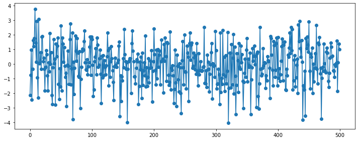
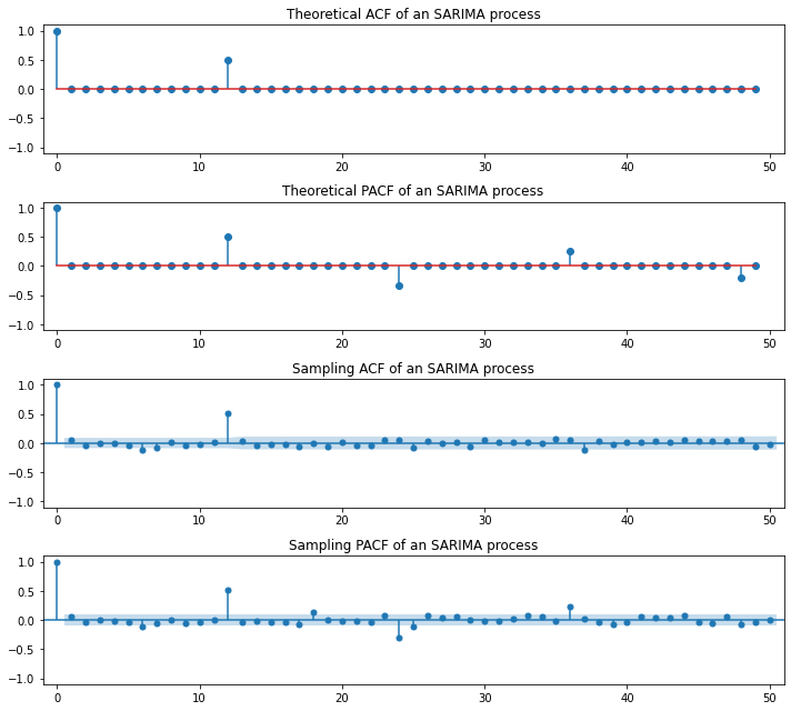
# SARIMA(0,0,0)(1,0,0,12)
plt.figure(figsize=(10, 4))
np.random.seed(123)
ar_params = np.array([0, 0, 0, 0, 0, 0, 0, 0, 0, 0, 0, 0.95])
ma_params = np.array([])
ar, ma = np.r_[1, -ar_params], np.r_[1, ma_params]
y = sm.tsa.ArmaProcess(ar, ma).generate_sample(500, burnin=50)
plt.plot(y, 'o-')
plt.tight_layout()
plt.show()

plt.figure(figsize=(10, 9))
plt.subplot(411)
plt.stem(sm.tsa.ArmaProcess(ar, ma).acf(lags=50))
plt.xlim(-1, 51)
plt.ylim(-1.1, 1.1)
plt.title("Theoretical ACF of an SARIMA process")

plt.subplot(412)
plt.stem(sm.tsa.ArmaProcess(ar, ma).pacf(lags=50))
plt.xlim(-1, 51)
plt.ylim(-1.1, 1.1)
plt.title("Theoretical PACF of an SARIMA process")

sm.graphics.tsa.plot_acf(y, lags=50, ax=plt.subplot(413))
plt.xlim(-1, 51)
plt.ylim(-1.1, 1.1)
plt.title("Sampling ACF of an SARIMA process")

sm.graphics.tsa.plot_pacf(y, lags=50, ax=plt.subplot(414))
plt.xlim(-1, 51)
plt.ylim(-1.1, 1.1)
plt.title("Sampling PACF of an SARIMA process")
plt.tight_layout()
plt.show()
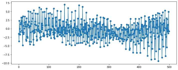
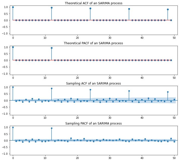
# SARIMA(0,0,0)(0,1,1,12)
plt.figure(figsize=(10, 4))
np.random.seed(123)
ar_params = np.array([0, 0, 0, 0, 0, 0, 0, 0, 0, 0, 0, 0.99])
ma_params = np.array([0, 0, 0, 0, 0, 0, 0, 0, 0, 0, 0, 0.95])
ar, ma = np.r_[1, -ar_params], np.r_[1, ma_params]
y = sm.tsa.ArmaProcess(ar, ma).generate_sample(500, burnin=50)
plt.plot(y, 'o-')
plt.tight_layout()
plt.show()

plt.figure(figsize=(10, 9))
plt.subplot(411)
plt.stem(sm.tsa.ArmaProcess(ar, ma).acf(lags=50))
plt.xlim(-1, 51)
plt.ylim(-1.1, 1.1)
plt.title("Theoretical ACF of an SARIMA process")

plt.subplot(412)
plt.stem(sm.tsa.ArmaProcess(ar, ma).pacf(lags=50))
plt.xlim(-1, 51)
plt.ylim(-1.1, 1.1)
plt.title("Theoretical PACF of an SARIMA process")

sm.graphics.tsa.plot_acf(y, lags=50, ax=plt.subplot(413))
plt.xlim(-1, 51)
plt.ylim(-1.1, 1.1)
plt.title("Sampling ACF of an SARIMA process")

sm.graphics.tsa.plot_pacf(y, lags=50, ax=plt.subplot(414))
plt.xlim(-1, 51)
plt.ylim(-1.1, 1.1)
plt.title("Sampling PACF of an SARIMA process")
plt.tight_layout()
plt.show()
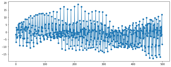
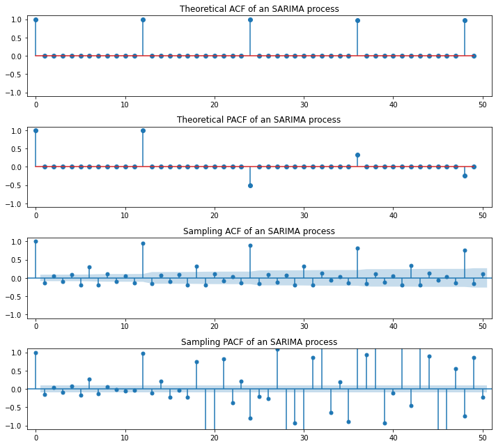
# SARIMA(0,0,0)(1,1,0,12)
plt.figure(figsize=(10, 4))
np.random.seed(123)
ar_params = np.array([0, 0, 0, 0, 0, 0, 0, 0, 0, 0, 0, 0.99, 0, 0, 0, 0, 0, 0, 0, 0, 0, 0, 0, -0.95])
ma_params = np.array([])
ar, ma = np.r_[1, -ar_params], np.r_[1, ma_params]
y = sm.tsa.ArmaProcess(ar, ma).generate_sample(500, burnin=50)
plt.plot(y, 'o-')
plt.tight_layout()
plt.show()

plt.figure(figsize=(10, 9))
plt.subplot(411)
plt.stem(sm.tsa.ArmaProcess(ar, ma).acf(lags=50))
plt.xlim(-1, 51)
plt.ylim(-1.1, 1.1)
plt.title("Theoretical ACF of an SARIMA process")

plt.subplot(412)
plt.stem(sm.tsa.ArmaProcess(ar, ma).pacf(lags=50))
plt.xlim(-1, 51)
plt.ylim(-1.1, 1.1)
plt.title("Theoretical PACF of an SARIMA process")

sm.graphics.tsa.plot_acf(y, lags=50, ax=plt.subplot(413))
plt.xlim(-1, 51)
plt.ylim(-1.1, 1.1)
plt.title("Sampling ACF of an SARIMA process")

sm.graphics.tsa.plot_pacf(y, lags=50, ax=plt.subplot(414))
plt.xlim(-1, 51)
plt.ylim(-1.1, 1.1)
plt.title("Sampling PACF of an SARIMA process")
plt.tight_layout()
plt.show()
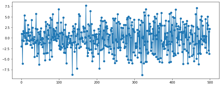
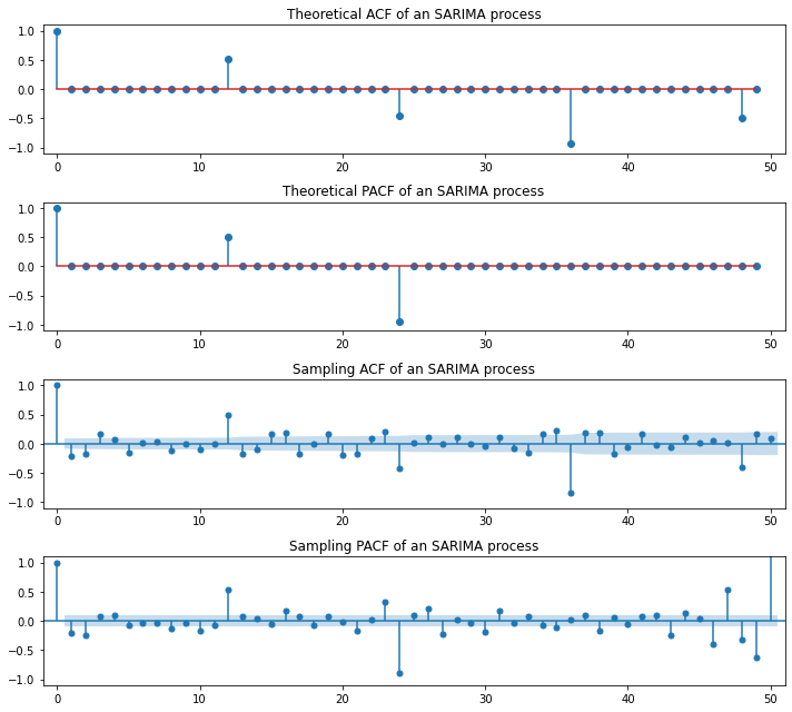
Multiplicated SARIMA: 계절성 시차와 그 주변의 시차에서도 ACF가 유의하지 않음
SARIMA(0,0,1)(0,0,1,12): 계절주기 12고 계절주기 자료들 간에는 ARIMA(0,0,1), 비계절 자료들 간에는 ARIMA(0,0,1)
시차(Lag)가 1, 11, 12, 13인 경우를 제외하고는 자기상관계수가 모두 0
\begin{align*} \text{Main Equation} && Y_t &= (1+\theta L)(1+\Theta L^{12}) \epsilon_t = \epsilon_t + \theta \epsilon_{t-1} + \Theta \epsilon_{t-12} + \theta\Theta \epsilon_{t-13} \ \text{Autocorrelation} && \rho_1 &= -\dfrac{\theta}{1+\theta^2} \ && \rho_{11} = \rho_{13} &= \dfrac{\theta\Theta}{(1+\theta^2)(1+\Theta^2)} \ && \rho_{12} &= -\dfrac{\Theta}{1+\Theta^2} \ \end{align*}
SARIMA(0,0,1)(1,0,0,12): 계절주기 12고 계절주기 자료들 간에는 ARIMA(1,0,0), 비계절 자료들 간에는 ARIMA(0,0,1)
시차(Lag)가 12의 배수와 그 앞/뒤인 경우(12\(k\), 12\(k\)+1, 12\(k\)-1)를 제외하고는 자기상관계수가 모두 0
\begin{align*} \text{Main Equation} && (1 - \Phi L^{12})Y_t &= (1 + \theta L) \epsilon_t \ && Y_t &= \Phi Y_{t-12} + \epsilon_t + \theta \epsilon_{t-1} \ \text{Autocorrelation} && \rho_{12k} &= (-1)^{k+1}\Phi^k \ && \rho_1 &= -\dfrac{\theta}{1+\theta^2} \ && \rho_{12k-1} = \rho_{12k+1} &= (-1)^{k+1}\dfrac{\theta}{1+\theta^2} \Phi^k \ \end{align*}
SARIMA(0,1,0)(0,1,0,12): 계절주기 12고 계절주기 간 1차 차분 ARIMA(0,0,0), 비계절 자료들 간 1차 차분 ARIMA(0,0,0)
시계열을 1차 차분하고 그 시계열을 다시 12간격 차분하면 백색잡음
\begin{align*} \text{Main Equation} && (1 - L^{12})(1 - L)Y_t &= \epsilon_t \ && (1 - L^{12})(Y_t - Y_{t-1}) &= \epsilon_t \ && Y_t - Y_{t-1} - Y_{t-12} + Y_{t-13} &= \epsilon_t \ && Y_t &= Y_{t-1} + Y_{t-12} - Y_{t-13} + \epsilon_t \ \end{align*}
SARIMA(0,1,1)(0,1,1,12): 계절주기 12고 계절/비계절 자료 모두 1차 차분 ARIMA(0,1,1)
시계열을 1차 차분하고 그 시계열을 다시 12간격 차분하면 계절/비계절 자료 모두 ARIMA(0,0,1)
\begin{align*} \text{Main Equation} && (1 - L^{12})(1 - L)Y_t &= (1 + \theta L)(1 + \Theta L^{12}) \epsilon_t \ && (1 - L^{12})(Y_t - Y_{t-1}) &= \epsilon_t + \theta \epsilon_{t-1} + \Theta \epsilon_{t-12} + \theta\Theta \epsilon_{t-13} \ && Y_t - Y_{t-1} - Y_{t-12} + Y_{t-13} &= \epsilon_t + \theta \epsilon_{t-1} + \Theta \epsilon_{t-12} + \theta\Theta \epsilon_{t-13} \ && Y_t &= Y_{t-1} + Y_{t-12} - Y_{t-13} + \epsilon_t + \theta \epsilon_{t-1} + \Theta \epsilon_{t-12} + \theta\Theta \epsilon_{t-13} \ \end{align*}
SARIMA(1,1,0)(1,1,0,12): 계절주기 12고 계절/비계절 자료 모두 1차 차분 ARIMA(1,1,0)
시계열을 1차 차분하고 그 시계열을 다시 12간격 차분하면 계절/비계절 자료 모두 ARIMA(1,0,0)
\begin{align*} \text{Main Equation} && (1 - \phi L)(1 - \Phi L^{12})(1 - L^{12})(1 - L)Y_t &= \epsilon_t \ && (1 - \phi L)(1 - \Phi L^{12})(1 - L^{12})(Y_t - Y_{t-1}) &= \epsilon_t \ && (1 - \phi L)(1 - \Phi L^{12})(Y_t - Y_{t-1} - Y_{t-12} + Y_{t-13}) &= \epsilon_t \ && (1 - \phi L)(Y_t - Y_{t-1} - Y_{t-12} + Y_{t-13} - \Phi Y_{t-12} + \Phi Y_{t-13} + \Phi Y_{t-24} - \Phi Y_{t-25}) Y_t &= \epsilon_t \ && (1 - \phi L)(Y_t - Y_{t-1} - (1 + \Phi)Y_{t-12} + (1 + \Phi)Y_{t-13} + \Phi Y_{t-24} - \Phi Y_{t-25}) Y_t &= \epsilon_t \ && Y_t - Y_{t-1} - (1 + \Phi)Y_{t-12} + (1 + \Phi)Y_{t-13} + \Phi Y_{t-24} - \Phi Y_{t-25} &\ && - \phi Y_{t-1} +\phi Y_{t-2} +\phi (1 + \Phi)Y_{t-13} -\phi (1 + \Phi)Y_{t-14} -\phi \Phi Y_{t-25} +\phi \Phi Y_{t-26} &= \epsilon_t \ && Y_t - (1+\phi) Y_{t-1} +\phi Y_{t-2} - (1 + \Phi)Y_{t-12} +((1 + \Phi)+\phi (1 + \Phi))Y_{t-13} &\ && -\phi (1 + \Phi)Y_{t-14} + \Phi Y_{t-24} - (\Phi+\phi \Phi) Y_{t-25} +\phi \Phi Y_{t-26} &= \epsilon_t \ \end{align*}
예시:
(원 데이터)
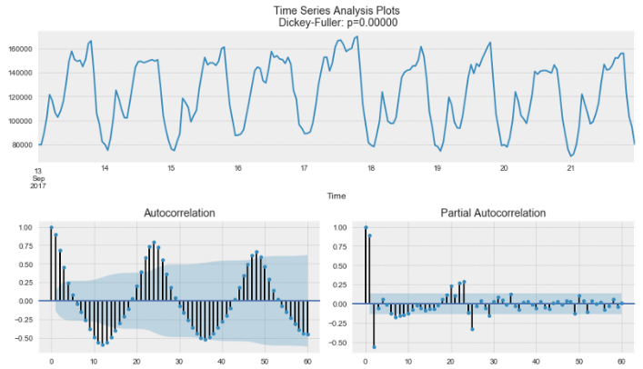
\(p:2?\) (PACF 기준 lag 2까지 유의하고 그 뒤로는 유의하지 않음)
\(d:1?\) (ADF가 대중가설을 기각하므로 추세 1차 차분)
\(q:1?\) (ACF 기준 필요성 인지)
\(P:1?\) (PACF 기준 lag 24 간격 유의성으로 필요성 인지)
\(D:1?\) (계절성 차분 필요함 인지)
\(Q:2?\) (ACF 기준 lag 24 간격 유의성으로 필요성 인지)
\(m:24?\) (ACF/PACF 기준 lag 24 간격으로 유의한 진동 존재)
(계절차분 후 데이터)
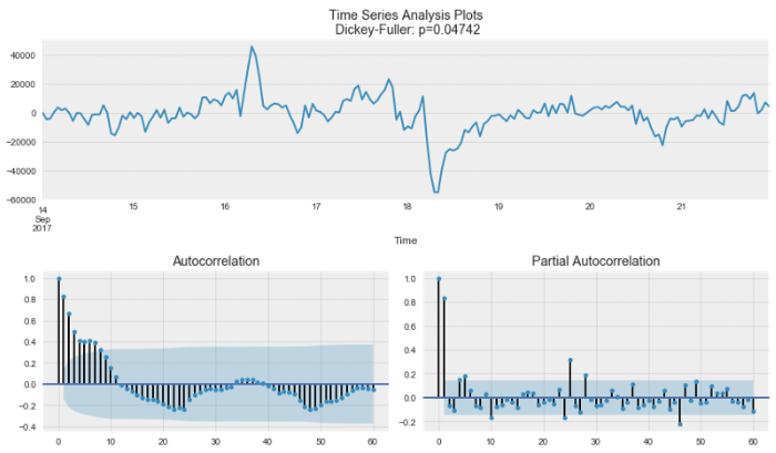
\(p:1?\) (PACF 기준 lag 1까지 유의하고 그 뒤로는 유의하지 않음)
\(d:1?\) (ADF가 대중가설을 기각하고 그래프 상 추세가 보이므로 일단 추세 1차 차분)
\(q:3?\) (ACF 기준 필요성 인지)
\(P:2?\) (PACF 기준 lag 24 간격 유의성으로 필요성 인지)
\(D:1\) (계절성 차분 필요)
\(Q:0?\) (ACF 기준 lag 24 간격 유의성으로 필요성 인지)
\(m:24\) (ACF/PACF 기준 lag 24 간격으로 유의한 진동 크게 사라짐)
(계절성 및 추세차분 후 데이터)
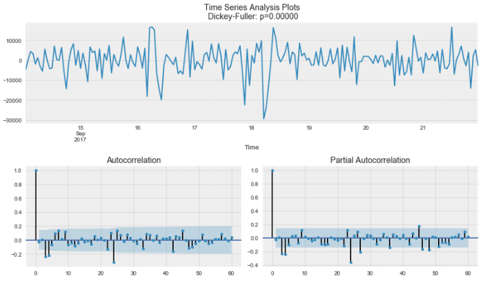
\(p:max4\) (PACF 기준 lag 4까지 유의하고 그 뒤로는 유의하지 않음)
\(d:1\) (ADF가 대중가설을 기각하고 그래프 상 추세도 없어졌으므로 추세 1차 차분 확정)
\(q:max4\) (ACF 기준 lag 4까지 유의하고 그 뒤로는 유의하지 않음)
\(P:max2\) (PACF 기준 lag 24 간격으로 2번정도 유의함)
\(D:1\) (계절성 차분 필요함 인지)
\(Q:max1\) (ACF 기준 lag 24 간격으로 1번정도 유의함)
\(m:24\) (lag 24 간격으로 진동 존재)
(잔차검증)
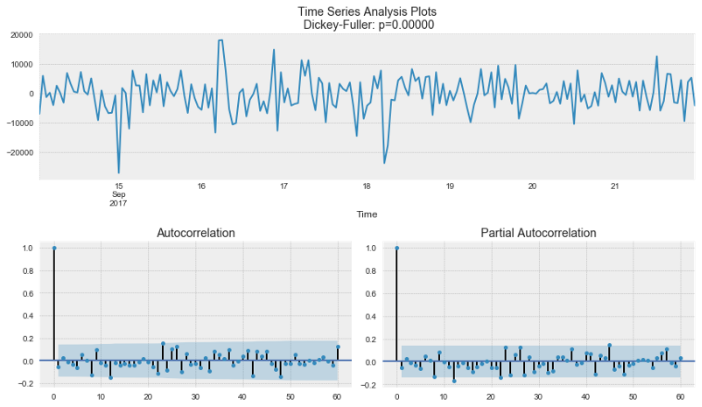
# SARIMA(0,0,1)(0,0,1,12)
plt.figure(figsize=(10, 4))
np.random.seed(123)
phi, Phi = 0, 0
theta, Theta = 0.5, 0.8
ar_params = np.array([])
ma_params = np.array([theta, 0, 0, 0, 0, 0, 0, 0, 0, 0, 0, Theta, theta*Theta])
ar, ma = np.r_[1, -ar_params], np.r_[1, ma_params]
y = sm.tsa.ArmaProcess(ar, ma).generate_sample(500, burnin=50)
plt.plot(y, 'o-')
plt.tight_layout()
plt.show()

plt.figure(figsize=(10, 9))
plt.subplot(411)
plt.stem(sm.tsa.ArmaProcess(ar, ma).acf(lags=50))
plt.xlim(-1, 51)
plt.ylim(-1.1, 1.1)
plt.title("Theoretical ACF of an SARIMA process")

plt.subplot(412)
plt.stem(sm.tsa.ArmaProcess(ar, ma).pacf(lags=50))
plt.xlim(-1, 51)
plt.ylim(-1.1, 1.1)
plt.title("Theoretical PACF of an SARIMA process")

sm.graphics.tsa.plot_acf(y, lags=50, ax=plt.subplot(413))
plt.xlim(-1, 51)
plt.ylim(-1.1, 1.1)
plt.title("Sampling ACF of an SARIMA process")

sm.graphics.tsa.plot_pacf(y, lags=50, ax=plt.subplot(414))
plt.xlim(-1, 51)
plt.ylim(-1.1, 1.1)
plt.title("Sampling PACF of an SARIMA process")
plt.tight_layout()
plt.show()
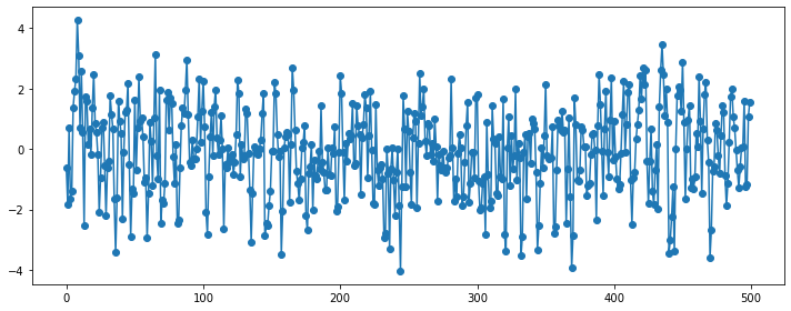
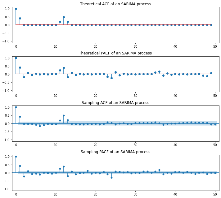
# SARIMA(0,0,1)(1,0,0,12)
plt.figure(figsize=(10, 4))
np.random.seed(123)
phi, Phi = 0, 0.75
theta, Theta = 0.5, 0
ar_params = np.array([0, 0, 0, 0, 0, 0, 0, 0, 0, 0, 0, Phi])
ma_params = np.array([theta])
ar, ma = np.r_[1, -ar_params], np.r_[1, ma_params]
y = sm.tsa.ArmaProcess(ar, ma).generate_sample(500, burnin=50)
plt.plot(y, 'o-')
plt.tight_layout()
plt.show()

plt.figure(figsize=(10, 9))
plt.subplot(411)
plt.stem(sm.tsa.ArmaProcess(ar, ma).acf(lags=50))
plt.xlim(-1, 51)
plt.ylim(-1.1, 1.1)
plt.title("Theoretical ACF of an SARIMA process")

plt.subplot(412)
plt.stem(sm.tsa.ArmaProcess(ar, ma).pacf(lags=50))
plt.xlim(-1, 51)
plt.ylim(-1.1, 1.1)
plt.title("Theoretical PACF of an SARIMA process")

sm.graphics.tsa.plot_acf(y, lags=50, ax=plt.subplot(413))
plt.xlim(-1, 51)
plt.ylim(-1.1, 1.1)
plt.title("Sampling ACF of an SARIMA process")

sm.graphics.tsa.plot_pacf(y, lags=50, ax=plt.subplot(414))
plt.xlim(-1, 51)
plt.ylim(-1.1, 1.1)
plt.title("Sampling PACF of an SARIMA process")
plt.tight_layout()
plt.show()
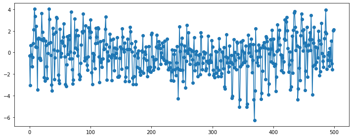
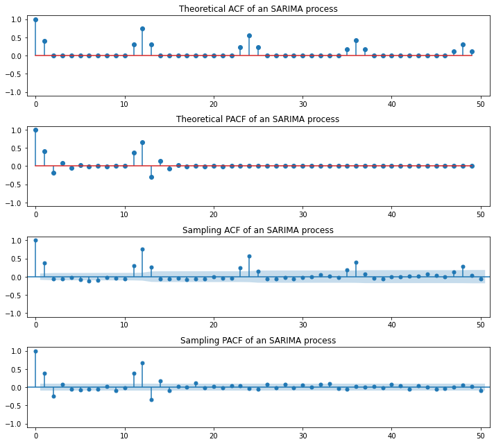
실습: 호흡기질환 사망자수 SARIMA 모델링
import warnings
warnings.filterwarnings('always')
warnings.filterwarnings('ignore')

import pandas as pd
import numpy as np
import matplotlib.pyplot as plt
import statsmodels.api as sm

# 데이터로딩 및 확인
data = sm.datasets.get_rdataset("deaths", "MASS")
raw = data.data
raw.value = np.log(raw.value)
raw.plot(x='time', y='value')
plt.show()

# ACF/PACF 확인
plt.figure(figsize=(10, 8))
sm.graphics.tsa.plot_acf(raw.value.values, lags=50, ax=plt.subplot(211))
plt.xlim(-1, 51)
plt.ylim(-1.1, 1.1)
plt.title("ACF")

sm.graphics.tsa.plot_pacf(raw.value.values, lags=50, ax=plt.subplot(212))
plt.xlim(-1, 51)
plt.ylim(-1.1, 1.1)
plt.title("PACF")
plt.tight_layout()
plt.show()

# ARMA(1,1) 모델링
fit = sm.tsa.SARIMAX(raw.value, trend='c', order=(1,0,1), seasonal_order=(0,0,0,0)).fit()
display(fit.summary())

# 잔차진단
fit.plot_diagnostics(figsize=(10,8))
plt.tight_layout()
plt.show()
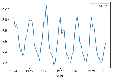
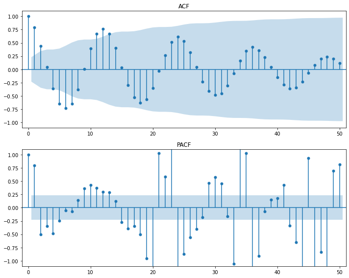
| Dep. Variable: | value | No. Observations: | 72 |
|---|---|---|---|
| Model: | SARIMAX(1, 0, 1) | Log Likelihood | 31.982 |
| Date: | Fri, 31 Jul 2020 | AIC | -55.965 |
| Time: | 22:46:34 | BIC | -46.858 |
| Sample: | 0 | HQIC | -52.339 |
| - 72 | |||
| Covariance Type: | opg |
| coef | std err | z | P>|z| | [0.025 | 0.975] | |
|---|---|---|---|---|---|---|
| intercept | 2.4194 | 0.765 | 3.161 | 0.002 | 0.919 | 3.920 |
| ar.L1 | 0.6818 | 0.100 | 6.846 | 0.000 | 0.487 | 0.877 |
| ma.L1 | 0.4668 | 0.116 | 4.027 | 0.000 | 0.240 | 0.694 |
| sigma2 | 0.0236 | 0.004 | 5.416 | 0.000 | 0.015 | 0.032 |
| Ljung-Box (Q): | 161.08 | Jarque-Bera (JB): | 12.13 |
|---|---|---|---|
| Prob(Q): | 0.00 | Prob(JB): | 0.00 |
| Heteroskedasticity (H): | 1.00 | Skew: | 0.94 |
| Prob(H) (two-sided): | 0.99 | Kurtosis: | 3.73 |
Warnings:
[1] Covariance matrix calculated using the outer product of gradients (complex-step).
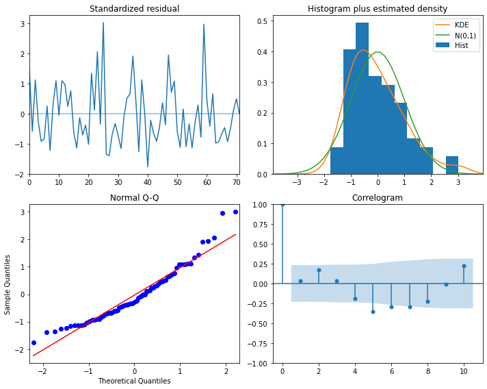
# SARIMA 모델링
fit = sm.tsa.SARIMAX(raw.value, trend='c', order=(1,0,1), seasonal_order=(1,1,1,12)).fit()
display(fit.summary())

# 잔차진단
fit.plot_diagnostics(figsize=(10,8))
plt.tight_layout()
plt.show()
| Dep. Variable: | value | No. Observations: | 72 |
|---|---|---|---|
| Model: | SARIMAX(1, 0, 1)x(1, 1, 1, 12) | Log Likelihood | 52.592 |
| Date: | Fri, 31 Jul 2020 | AIC | -93.184 |
| Time: | 22:46:36 | BIC | -80.618 |
| Sample: | 0 | HQIC | -88.269 |
| - 72 | |||
| Covariance Type: | opg |
| coef | std err | z | P>|z| | [0.025 | 0.975] | |
|---|---|---|---|---|---|---|
| intercept | -0.0480 | 0.022 | -2.211 | 0.027 | -0.091 | -0.005 |
| ar.L1 | -0.1563 | 0.436 | -0.359 | 0.720 | -1.010 | 0.698 |
| ma.L1 | 0.5718 | 0.273 | 2.097 | 0.036 | 0.037 | 1.106 |
| ar.S.L12 | -0.2861 | 0.203 | -1.406 | 0.160 | -0.685 | 0.113 |
| ma.S.L12 | -0.9670 | 4.319 | -0.224 | 0.823 | -9.431 | 7.497 |
| sigma2 | 0.0066 | 0.028 | 0.239 | 0.811 | -0.047 | 0.061 |
| Ljung-Box (Q): | 28.57 | Jarque-Bera (JB): | 74.39 |
|---|---|---|---|
| Prob(Q): | 0.91 | Prob(JB): | 0.00 |
| Heteroskedasticity (H): | 0.64 | Skew: | 0.99 |
| Prob(H) (two-sided): | 0.32 | Kurtosis: | 8.08 |
Warnings:
[1] Covariance matrix calculated using the outer product of gradients (complex-step).
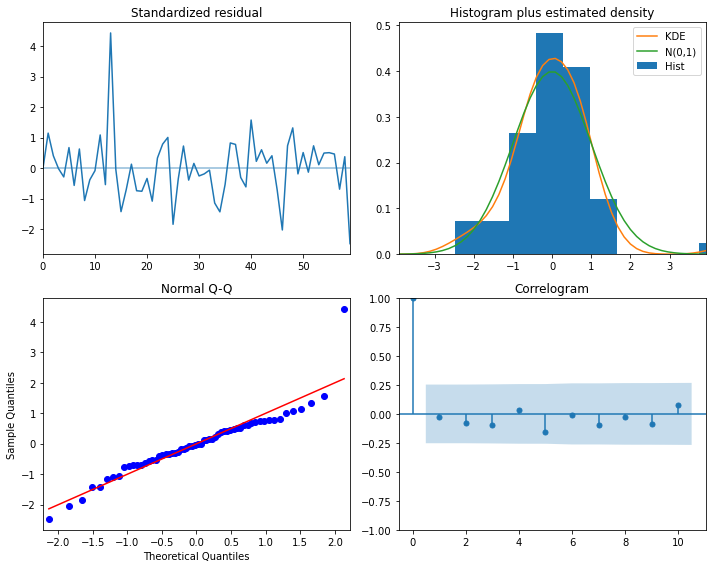
실습: 항공사 승객수요 SARIMA 모델링
# 라이브러리 호출
import pandas as pd
import numpy as np
import matplotlib.pyplot as plt
import statsmodels.api as sm

# 데이터 준비
data = sm.datasets.get_rdataset("AirPassengers")
raw = data.data.copy()

# 데이터 전처리
## 시간 인덱싱
if 'time' in raw.columns:
    raw.index = pd.date_range(start='1/1/1949', periods=len(raw['time']), freq='M')
    del raw['time']

## 정상성 확보
plt.figure(figsize=(12,8))
raw.plot(ax=plt.subplot(221), title='Y', legend=False)
np.log(raw).plot(ax=plt.subplot(222), title='log(Y)', legend=False)
raw.diff(1).plot(ax=plt.subplot(223), title='diff1(Y)', legend=False)
np.log(raw).diff(1).plot(ax=plt.subplot(224), title='diff1(log(Y))', legend=False)
plt.show()
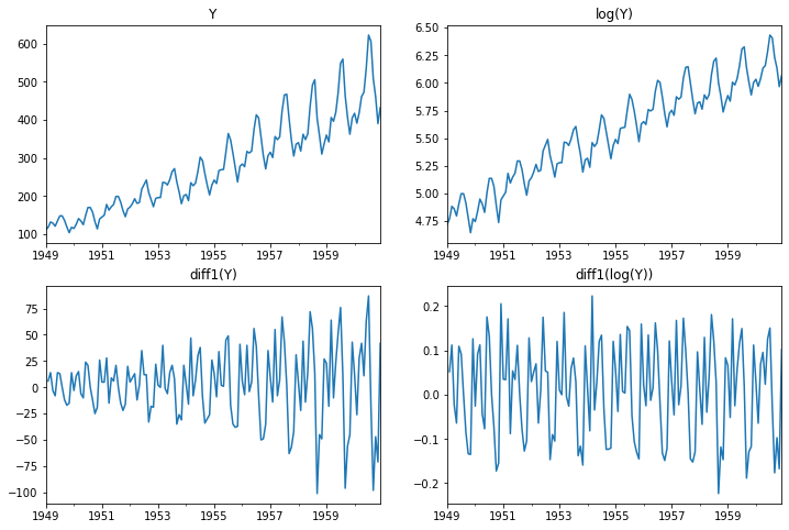
# ARIMA 모델링 (raw)
fit = sm.tsa.SARIMAX(raw.value, trend='c', order=(1,1,1), seasonal_order=(0,0,0,0)).fit()
display(fit.summary())

# 잔차진단
fit.plot_diagnostics(figsize=(10,8))
plt.tight_layout()
plt.show()

# ARIMA 모델링 (log(raw))
fit = sm.tsa.SARIMAX(np.log(raw.value), trend='c', order=(1,1,1), seasonal_order=(0,0,0,0)).fit()
display(fit.summary())

# 잔차진단
fit.plot_diagnostics(figsize=(10,8))
plt.tight_layout()
plt.show()
| Dep. Variable: | value | No. Observations: | 144 |
|---|---|---|---|
| Model: | SARIMAX(1, 1, 1) | Log Likelihood | -694.060 |
| Date: | Fri, 31 Jul 2020 | AIC | 1396.121 |
| Time: | 22:46:41 | BIC | 1407.972 |
| Sample: | 01-31-1949 | HQIC | 1400.937 |
| - 12-31-1960 | |||
| Covariance Type: | opg |
| coef | std err | z | P>|z| | [0.025 | 0.975] | |
|---|---|---|---|---|---|---|
| intercept | 3.6187 | 5.001 | 0.724 | 0.469 | -6.183 | 13.421 |
| ar.L1 | -0.4768 | 0.128 | -3.736 | 0.000 | -0.727 | -0.227 |
| ma.L1 | 0.8646 | 0.080 | 10.746 | 0.000 | 0.707 | 1.022 |
| sigma2 | 958.4116 | 107.040 | 8.954 | 0.000 | 748.616 | 1168.207 |
| Ljung-Box (Q): | 318.10 | Jarque-Bera (JB): | 2.17 |
|---|---|---|---|
| Prob(Q): | 0.00 | Prob(JB): | 0.34 |
| Heteroskedasticity (H): | 7.01 | Skew: | -0.21 |
| Prob(H) (two-sided): | 0.00 | Kurtosis: | 3.43 |
Warnings:
[1] Covariance matrix calculated using the outer product of gradients (complex-step).
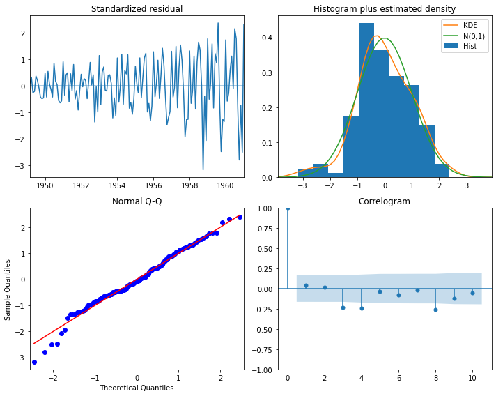
| Dep. Variable: | value | No. Observations: | 144 |
|---|---|---|---|
| Model: | SARIMAX(1, 1, 1) | Log Likelihood | 124.804 |
| Date: | Fri, 31 Jul 2020 | AIC | -241.608 |
| Time: | 22:46:41 | BIC | -229.756 |
| Sample: | 01-31-1949 | HQIC | -236.792 |
| - 12-31-1960 | |||
| Covariance Type: | opg |
| coef | std err | z | P>|z| | [0.025 | 0.975] | |
|---|---|---|---|---|---|---|
| intercept | 0.0155 | 0.016 | 0.963 | 0.336 | -0.016 | 0.047 |
| ar.L1 | -0.5826 | 0.170 | -3.430 | 0.001 | -0.915 | -0.250 |
| ma.L1 | 0.8502 | 0.101 | 8.454 | 0.000 | 0.653 | 1.047 |
| sigma2 | 0.0102 | 0.002 | 5.871 | 0.000 | 0.007 | 0.014 |
| Ljung-Box (Q): | 355.82 | Jarque-Bera (JB): | 5.93 |
|---|---|---|---|
| Prob(Q): | 0.00 | Prob(JB): | 0.05 |
| Heteroskedasticity (H): | 1.07 | Skew: | 0.04 |
| Prob(H) (two-sided): | 0.81 | Kurtosis: | 2.01 |
Warnings:
[1] Covariance matrix calculated using the outer product of gradients (complex-step).
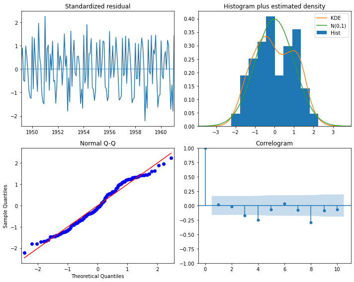
# SARIMA 모델링 (log(raw))
fit = sm.tsa.SARIMAX(np.log(raw.value), trend='c', order=(1,1,1), seasonal_order=(1,1,1,12)).fit()
display(fit.summary())

# 잔차진단
fit.plot_diagnostics(figsize=(10,8))
plt.tight_layout()
plt.show()
| Dep. Variable: | value | No. Observations: | 144 |
|---|---|---|---|
| Model: | SARIMAX(1, 1, 1)x(1, 1, 1, 12) | Log Likelihood | 245.172 |
| Date: | Fri, 31 Jul 2020 | AIC | -478.344 |
| Time: | 22:46:44 | BIC | -461.093 |
| Sample: | 01-31-1949 | HQIC | -471.334 |
| - 12-31-1960 | |||
| Covariance Type: | opg |
| coef | std err | z | P>|z| | [0.025 | 0.975] | |
|---|---|---|---|---|---|---|
| intercept | -0.0002 | 0.001 | -0.192 | 0.848 | -0.002 | 0.001 |
| ar.L1 | 0.1728 | 0.214 | 0.809 | 0.418 | -0.246 | 0.591 |
| ma.L1 | -0.5657 | 0.186 | -3.046 | 0.002 | -0.930 | -0.202 |
| ar.S.L12 | -0.0949 | 0.202 | -0.470 | 0.638 | -0.491 | 0.301 |
| ma.S.L12 | -0.5019 | 0.218 | -2.300 | 0.021 | -0.930 | -0.074 |
| sigma2 | 0.0013 | 0.000 | 8.474 | 0.000 | 0.001 | 0.002 |
| Ljung-Box (Q): | 37.14 | Jarque-Bera (JB): | 3.52 |
|---|---|---|---|
| Prob(Q): | 0.60 | Prob(JB): | 0.17 |
| Heteroskedasticity (H): | 0.61 | Skew: | -0.02 |
| Prob(H) (two-sided): | 0.10 | Kurtosis: | 3.80 |
Warnings:
[1] Covariance matrix calculated using the outer product of gradients (complex-step).
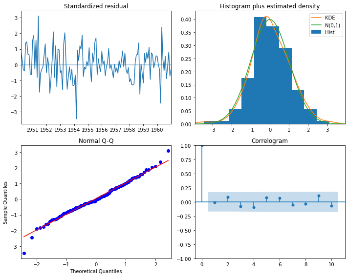
선형확률과정의 분석싸이클
분석싸이클 정리(Non-seasonal)
1. 분석싸이클 제시: <박스-젠킨스 방법론>
1) 모형의 모수추정(Model Identification): - 시계열 데이터의 정상성을 확인하고 계절변동이 있는지도 확인
- ACF/PACF 를 사용해서 자기회귀이동평균 모형 p,q 차수를 결정
2) 모델링 및 검증(Parameter Estimation):
- 회귀분석과 기계학습 등의 검증지표를 마찬가지로 사용
- 모형 추정은 최소제곱방법과 유사하지만 가우스-뉴튼 아이디어에 기초한 수치해석방법을 적용
3) 잔차진단(Model Diagnostics):
- 자기회귀이동평균 모형을 적용시키고 남은 잔차의 정상성을 확인하는데 중점
- 잔차가 서로 독립이고 시간에 따라 평균과 분산이 일정한지 검증 - 시계열 데이터의 자기상관을 검정하기 위해 다양한 검정통계량을 사용하는데,
Ljung-Box 통계량, 평균과 분산이 일정한지, ACF/PACF 사용하여 추가적으로 모형에 누락된 것이 없는지 검정
2. 분석싸이클 일반화
0) 데이터 전처리 및 시각화를 통해 Outlier 확인/변경/제거
1) 비정상 과정에서 정상 과정 추출
결정론적 추세나 확률적 추세가 있는지 확인
결정론적 추세는 회귀분석, 다항식 등으로 모형화 후 이를 분리
확률적 추세인 경우, 즉 ARIMA 모형인 경우에는 ADF(Augmented Dickey Fuller) 검정을 사용하여 적분차수(Order of Integration)을 알아내서 차분
2) 정규성 확인
정규성 검정을 통해 자료의 분포가 정규 분포인지 확인
일반 선형 확률 과정인 경우에는 전체 시계열이 가우시안 백색 잡음의 선형 조합으로 이루어지기 때문에 시계열 자체도 가우시안 정규 분포
ARIMA 모형 등의 일반 선형 확률 과정으로 모형화하려면 우선 정규성 검정(Normality Test)을 사용하여 분포가 정규 분포인지 확인
만약 시계열 자료의 분포가 로그 변환이나 Box-Cox 변환을 사용하여 정규성이 개선된다면 이러한 변환을 사용 가능
3) 정상 과정에 대한 ARMA 모형 차수 결정
ACF/PACF 분석으로 AR(p) 모형 또는 MA(q) 모형 결정
ACF가 특정 차수 이상에서 없어지는 경우(Cut-off)에는 MA 모형을 사용 가능
PACF가 특정 차수 이상에서 없어지면 AR 모형을 사용 가능
ACF와 PACF 모두 특정 차수 이상에서 없어지는 현상이 나타나지 않는다면 ARMA 모형을 사용
ARMA 모형인 경우 모수 추정시 AIC/BIC 값을 이용하여 차수 결정 및 모수추정도 동시에 이루어 짐
4) ARMA 모형의 모수 추정
MM(Method of Modent)/LS(Least Square)/MLE(Maximum Likelihood Estimation) 등의 방법론으로 모수 추정
ADF(Augmented Dickey Fuller) 검정을 사용하여 해당 수식에 대한 계수 즉 모수 값을 추정
부트스트래핑을 사용하여 모수의 표준 오차 추정
5) 잔차 진단(모형 진단)
: 모형이 추정된 다음 진단(Diagnosis) 과정을 통해 추정이 올바르게 이루어졌는지 검증
: 기본적으로 잔차(Residual)가 백색 잡음이 되어야 하므로 잔차에 대해 다음을 조사
잔차에 대한 정규성 검정
잔차에 대한 ACF 분석 또는 Ljung-Box Q 검정으로 모형 차수 재확인
: 잔차가 백색잡음이 아니면 새로운 모형으로 위 모든 단계(0~4단계)를 새로 시작
: 잔차가 백색잡음이면 일단은 예측력을 확인 -> 예측력이 낮을 시 새로운 모형으로 위 모든 단계(0~4단계)를 새로 시작
3. 분석싸이클 비교:
단계 |
기계학습 |
시계열분석 |
|---|---|---|
전처리 |
변수 확장 |
정상성 확보 |
시각화 |
모델/변수 선택 |
모델/파라미터 선택 |
모델링 |
상동 |
상동 |
검증 |
상동 |
상동 |
잔차진단 |
상동 |
상동 |
분석싸이클 자동화(Non-seasonal)
“Hyndman-Khandakar algorithm for automatic ARIMA modelling”
차수가 높지않은 SARIMA 알고리즘을 자동화 한 것으로 Hyndman-Khandakar 알고리즘(2008)을 기반으로 함
정상성변환(Unit Root Calculation), 검증지표 최적화(AIC) 및 MLE 방법을 사용한 모수추정을 모두 포함
자동화 과정: 일반화 분석싸이클의 2~4단계만 자동화
1. KPSS 검정통계량을 사용한 독립변수(\(Y_t\))의 적분차수/차분차수 결정(\(0 \leq d \leq 2\))
2. 차분된 독립변수 \((1 - L)^d Y_t\)에 \(AIC\)를 줄여가며 초기모형 후보들 적합을 통한 Base모형의 차수 \(p\)와 \(q\)를 선택
만약 \(d \leq 1\), 초기모형 후보 5종 - ARIMA(0,d,0) without constant - ARIMA(0,d,0) with constant - ARIMA(0,d,1) with constant - ARIMA(1,d,0) with constant - ARIMA(2,d,2) with constant
만약 \(d = 2\), 초기모형 후보 4종 - ARIMA(0,d,0) without constant - ARIMA(0,d,1) without constant - ARIMA(1,d,0) without constant - ARIMA(2,d,2) without constant
3. Base모형의 파라미터 튜닝을 통한 Agile모형 선택
Base모형에서 \(p\)와 \(q\)를 \(\pm 1\) 변화시키며 AIC들을 추정
\(p\)와 \(q\) 변경 및 상수항(Constant) 반영/미반영하며 AIC들을 추정
최적의 Agile모형 선택
4. 최종 모형 선택
추정된 Agile모형을 Base모형으로 변경
AIC가 더이상 줄어들지 않을 때까지 3번의 과정을 반복하여 Agile모형 재추정
최종 Agile모형이 최종 선택된 시계열모형
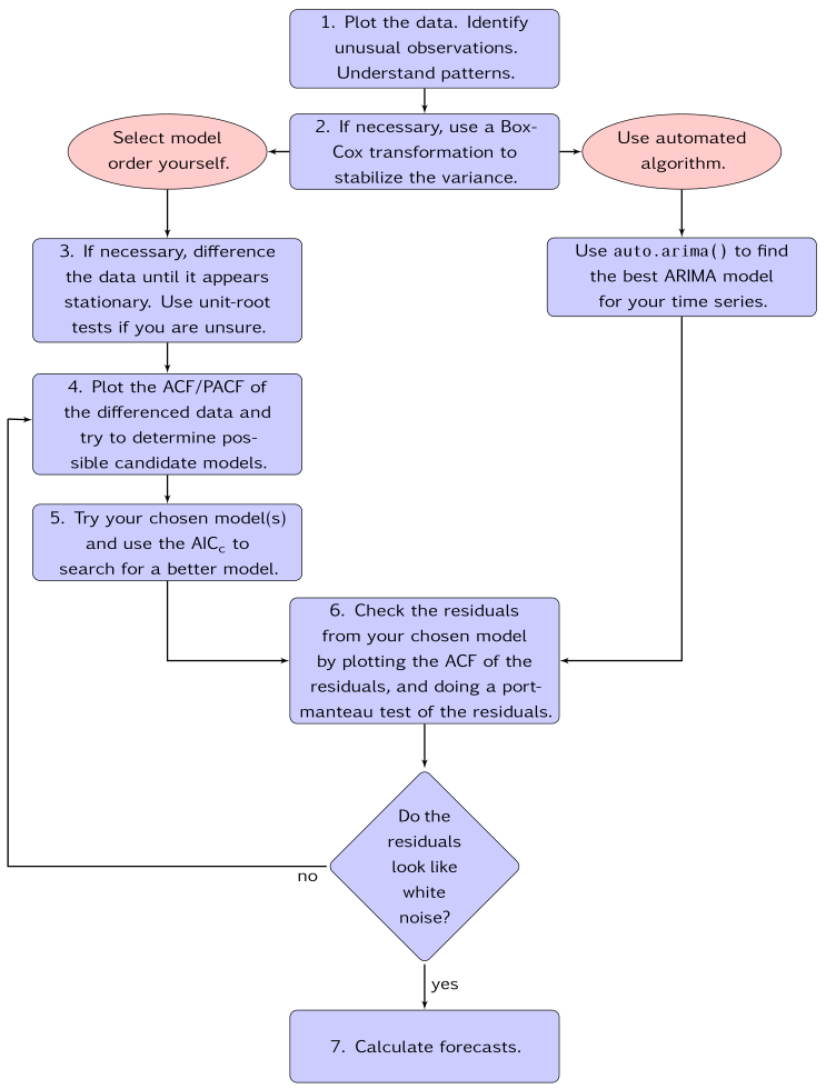
fit = auto_arima(Y_train, stationary=False,
                 trend='c', start_p=0, start_q=0, max_p=5, max_q=5, max_d=3,
                 seasonal=True, start_P=0, start_Q=0, max_P=5, max_Q=5, m=seasonal_diff_order,
                 stepwise=True, trace=True)
실습: 항공사 승객수요 Auro-ARIMA 모델링
# 라이브러리 호출
import pandas as pd
import numpy as np
import matplotlib.pyplot as plt
import statsmodels.api as sm
%reload_ext autoreload
%autoreload 2
from module import stationarity_adf_test, stationarity_kpss_test

# 데이터 준비
data = sm.datasets.get_rdataset("AirPassengers")
raw = data.data.copy()

# 데이터 전처리
## 시간 인덱싱
if 'time' in raw.columns:
    raw.index = pd.date_range(start='1/1/1949', periods=len(raw['time']), freq='M')
    del raw['time']

## 정상성 테스트
### 미변환
candidate_none = raw.copy()
display(stationarity_adf_test(candidate_none.values.flatten(), []))
display(stationarity_kpss_test(candidate_none.values.flatten(), []))
sm.graphics.tsa.plot_acf(candidate_none, lags=100, use_vlines=True)
plt.tight_layout()
plt.show()

### 로그 변환
candidate_trend = np.log(raw).copy()
display(stationarity_adf_test(candidate_trend.values.flatten(), []))
display(stationarity_kpss_test(candidate_trend.values.flatten(), []))
sm.graphics.tsa.plot_acf(candidate_trend, lags=100, use_vlines=True)
plt.tight_layout()
plt.show()

trend_diff_order_initial = 0
result = stationarity_adf_test(candidate_trend.values.flatten(), []).T
if result['p-value'].values.flatten() < 0.1:
    trend_diff_order = trend_diff_order_initial
else:
    trend_diff_order = trend_diff_order_initial + 1
print('Trend Difference: ', trend_diff_order)

### 로그+추세차분 변환
candidate_seasonal = candidate_trend.diff(trend_diff_order).dropna().copy()
display(stationarity_adf_test(candidate_seasonal.values.flatten(), []))
display(stationarity_kpss_test(candidate_seasonal.values.flatten(), []))
sm.graphics.tsa.plot_acf(candidate_seasonal, lags=100, use_vlines=True)
plt.tight_layout()
plt.show()

seasonal_diff_order = sm.tsa.acf(candidate_seasonal)[1:].argmax() + 1
print('Seasonal Difference: ', seasonal_diff_order)

### 로그+추세차분+계절차분 변환
candidate_final = candidate_seasonal.diff(seasonal_diff_order).dropna().copy()
display(stationarity_adf_test(candidate_final.values.flatten(), []))
display(stationarity_kpss_test(candidate_final.values.flatten(), []))
sm.graphics.tsa.plot_acf(candidate_final, lags=100, use_vlines=True)
plt.tight_layout()
plt.show()
| Stationarity_adf | |
|---|---|
| Test Statistics | 0.82 |
| p-value | 0.99 |
| Used Lag | 13.00 |
| Used Observations | 130.00 |
| Critical Value(1%) | -3.48 |
| Maximum Information Criteria | 996.69 |
| Stationarity_kpss | |
|---|---|
| Test Statistics | 1.05 |
| p-value | 0.01 |
| Used Lag | 14.00 |
| Critical Value(10%) | 0.35 |

| Stationarity_adf | |
|---|---|
| Test Statistics | -1.72 |
| p-value | 0.42 |
| Used Lag | 13.00 |
| Used Observations | 130.00 |
| Critical Value(1%) | -3.48 |
| Maximum Information Criteria | -445.40 |
| Stationarity_kpss | |
|---|---|
| Test Statistics | 1.05 |
| p-value | 0.01 |
| Used Lag | 14.00 |
| Critical Value(10%) | 0.35 |

Trend Difference: 1
| Stationarity_adf | |
|---|---|
| Test Statistics | -2.72 |
| p-value | 0.07 |
| Used Lag | 14.00 |
| Used Observations | 128.00 |
| Critical Value(1%) | -3.48 |
| Maximum Information Criteria | -440.36 |
| Stationarity_kpss | |
|---|---|
| Test Statistics | 0.10 |
| p-value | 0.10 |
| Used Lag | 14.00 |
| Critical Value(10%) | 0.35 |
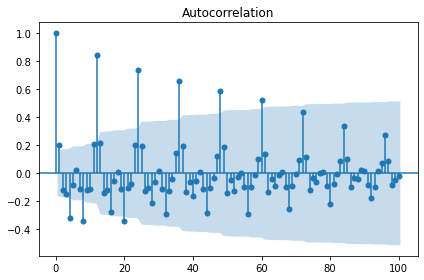
Seasonal Difference: 12
| Stationarity_adf | |
|---|---|
| Test Statistics | -4.44 |
| p-value | 0.00 |
| Used Lag | 12.00 |
| Used Observations | 118.00 |
| Critical Value(1%) | -3.49 |
| Maximum Information Criteria | -415.56 |
| Stationarity_kpss | |
|---|---|
| Test Statistics | 0.11 |
| p-value | 0.10 |
| Used Lag | 13.00 |
| Critical Value(10%) | 0.35 |

## 최종 타겟 선정 및 Train/Test 데이터 분리
candidate = candidate_trend.copy()
split_date = '1958-01-01'
Y_train = candidate[candidate.index < split_date]
Y_test = candidate[candidate.index >= split_date]

## 시각화 및 모수추론(p=1, q=0, d=1, P=1, Q=1, D(m)=12)
plt.figure(figsize=(14,4))
sm.tsa.graphics.plot_acf(Y_train, lags=50, alpha=0.05, use_vlines=True, ax=plt.subplot(121))
sm.tsa.graphics.plot_pacf(Y_train, lags=50, alpha=0.05, use_vlines=True, ax=plt.subplot(122))
plt.show()

# 모델링
## SARIMAX
logarithm, differencing = True, False
# fit_ts_sarimax = sm.tsa.SARIMAX(Y_train, order=(1,trend_diff_order,0), trend='ct').fit()
# fit_ts_sarimax = sm.tsa.SARIMAX(Y_train, order=(1,trend_diff_order,0),
#                                 seasonal_order=(0,0,1,seasonal_diff_order), trend='c').fit()
# fit_ts_sarimax = sm.tsa.SARIMAX(Y_train, order=(1,trend_diff_order,0),
#                                 seasonal_order=(1,0,0,seasonal_diff_order), trend='c').fit()
fit_ts_sarimax = sm.tsa.SARIMAX(Y_train, order=(1,trend_diff_order,0),
                                seasonal_order=(1,0,1,seasonal_diff_order), trend='c').fit()
display(fit_ts_sarimax.summary())
pred_tr_ts_sarimax = fit_ts_sarimax.predict()
pred_te_ts_sarimax = fit_ts_sarimax.get_forecast(len(Y_test)).predicted_mean
pred_te_ts_sarimax_ci = fit_ts_sarimax.get_forecast(len(Y_test)).conf_int()
## 비정상성으로 변환
if logarithm:
    Y_train = np.exp(Y_train).copy()
    Y_test = np.exp(Y_test).copy()
    pred_tr_ts_sarimax = np.exp(pred_tr_ts_sarimax).copy()
    pred_te_ts_sarimax = np.exp(pred_te_ts_sarimax).copy()
    pred_te_ts_sarimax_ci = np.exp(pred_te_ts_sarimax_ci).copy()
if differencing:
    pred_tr_ts_sarimax = np.cumsum(pred_tr_ts_sarimax).copy()

# 검증
%reload_ext autoreload
%autoreload 2
from module import *
Score_ts_sarimax, Resid_tr_ts_sarimax, Resid_te_ts_sarimax = evaluation_trte(Y_train, pred_tr_ts_sarimax,
                                                                             Y_test, pred_te_ts_sarimax, graph_on=True)
display(Score_ts_sarimax)
ax = pd.DataFrame(Y_test).plot(figsize=(12,4))
pd.DataFrame(pred_te_ts_sarimax, index=Y_test.index, columns=['prediction']).plot(kind='line',
                                                                           xlim=(Y_test.index.min(),Y_test.index.max()),
                                                                           linewidth=3, fontsize=20, ax=ax)
ax.fill_between(pd.DataFrame(pred_te_ts_sarimax_ci, index=Y_test.index).index,
                pd.DataFrame(pred_te_ts_sarimax_ci, index=Y_test.index).iloc[:,0],
                pd.DataFrame(pred_te_ts_sarimax_ci, index=Y_test.index).iloc[:,1], color='k', alpha=0.15)
plt.show()

# 잔차진단
error_analysis(Resid_tr_ts_sarimax, ['Error'], Y_train, graph_on=True)
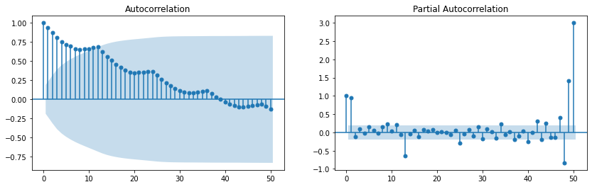
| Dep. Variable: | value | No. Observations: | 108 |
|---|---|---|---|
| Model: | SARIMAX(1, 1, 0)x(1, 0, [1], 12) | Log Likelihood | 184.253 |
| Date: | Fri, 31 Jul 2020 | AIC | -358.506 |
| Time: | 22:46:49 | BIC | -345.142 |
| Sample: | 01-31-1949 | HQIC | -353.089 |
| - 12-31-1957 | |||
| Covariance Type: | opg |
| coef | std err | z | P>|z| | [0.025 | 0.975] | |
|---|---|---|---|---|---|---|
| intercept | 0.0001 | 0.000 | 0.330 | 0.741 | -0.001 | 0.001 |
| ar.L1 | -0.2676 | 0.080 | -3.352 | 0.001 | -0.424 | -0.111 |
| ar.S.L12 | 0.9907 | 0.008 | 120.894 | 0.000 | 0.975 | 1.007 |
| ma.S.L12 | -0.6113 | 0.114 | -5.341 | 0.000 | -0.836 | -0.387 |
| sigma2 | 0.0014 | 0.000 | 7.243 | 0.000 | 0.001 | 0.002 |
| Ljung-Box (Q): | 40.18 | Jarque-Bera (JB): | 0.23 |
|---|---|---|---|
| Prob(Q): | 0.46 | Prob(JB): | 0.89 |
| Heteroskedasticity (H): | 0.39 | Skew: | 0.09 |
| Prob(H) (two-sided): | 0.01 | Kurtosis: | 3.15 |
Warnings:
[1] Covariance matrix calculated using the outer product of gradients (complex-step).
| MAE | MSE | MAPE | |
|---|---|---|---|
| Train | 8.27 | 197.76 | 4.53 |
| Test | 26.96 | 910.97 | 6.63 |
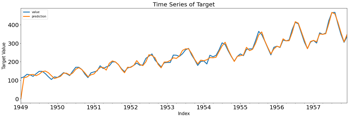
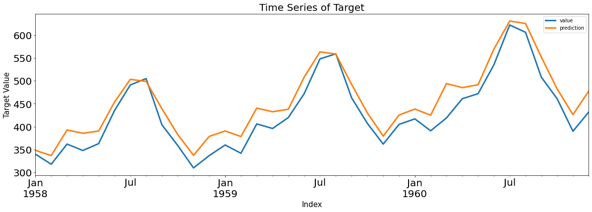
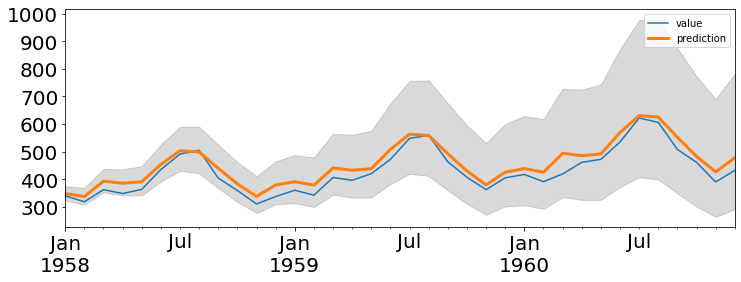
*c* argument looks like a single numeric RGB or RGBA sequence, which should be avoided as value-mapping will have precedence in case its length matches with *x* & *y*.  Please use the *color* keyword-argument or provide a 2-D array with a single row if you intend to specify the same RGB or RGBA value for all points.
*c* argument looks like a single numeric RGB or RGBA sequence, which should be avoided as value-mapping will have precedence in case its length matches with *x* & *y*.  Please use the *color* keyword-argument or provide a 2-D array with a single row if you intend to specify the same RGB or RGBA value for all points.
*c* argument looks like a single numeric RGB or RGBA sequence, which should be avoided as value-mapping will have precedence in case its length matches with *x* & *y*.  Please use the *color* keyword-argument or provide a 2-D array with a single row if you intend to specify the same RGB or RGBA value for all points.
*c* argument looks like a single numeric RGB or RGBA sequence, which should be avoided as value-mapping will have precedence in case its length matches with *x* & *y*.  Please use the *color* keyword-argument or provide a 2-D array with a single row if you intend to specify the same RGB or RGBA value for all points.
| Stationarity_adf | Stationarity_kpss | Normality | Autocorr(lag1) | Autocorr(lag5) | Autocorr(lag10) | Autocorr(lag50) | Heteroscedasticity | |
|---|---|---|---|---|---|---|---|---|
| Test Statistics | -7.45 | 0.33 | 0.69 | 0.34 | 4.17 | 12.70 | 29.56 | 0.23 |
| p-value | 0.00 | 0.10 | 0.00 | 0.56 | 0.53 | 0.24 | 0.99 | 0.00 |
| Used Lag | 3.00 | 13.00 | nan | nan | nan | nan | nan | NaN |
| Used Observations | 104.00 | nan | nan | nan | nan | nan | nan | NaN |
| Critical Value(1%) | -3.49 | nan | nan | nan | nan | nan | nan | NaN |
| Maximum Information Criteria | 677.41 | nan | nan | nan | nan | nan | nan | NaN |
| Critical Value(10%) | nan | 0.35 | nan | nan | nan | nan | nan | NaN |
| Alternative | nan | nan | nan | nan | nan | nan | nan | two-sided |
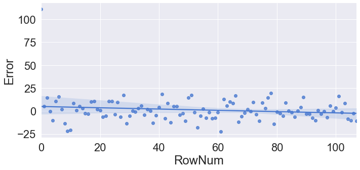
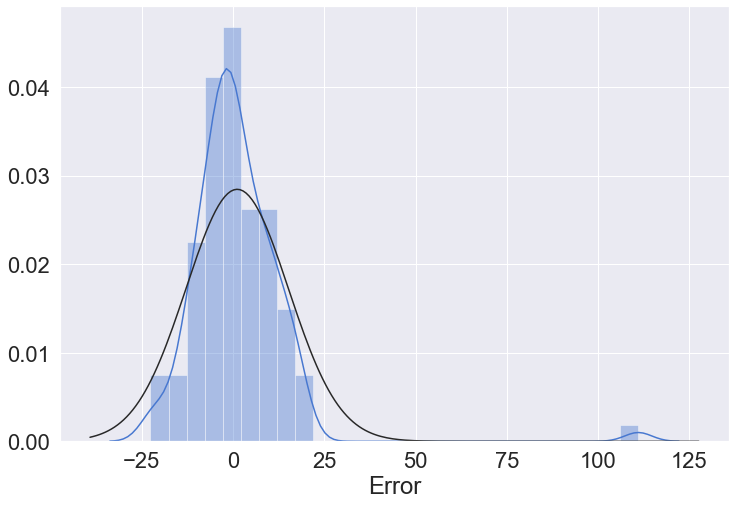
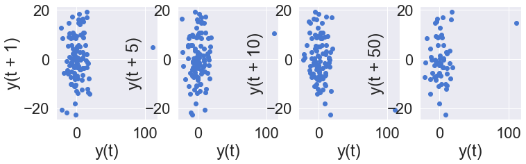
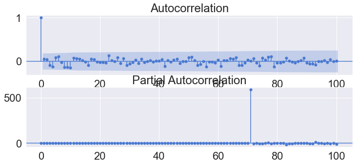
# ## 최종 타겟 선정 및 Train/Test 데이터 분리
# candidate = candidate_trend.copy()
# split_date = '1958-01-01'
# Y_train = candidate[candidate.index < split_date]
# Y_test = candidate[candidate.index >= split_date]

# ## 시각화 및 모수추론(p=1, q=0, d=1, P=1, Q=1, D(m)=12)
# plt.figure(figsize=(14,4))
# sm.tsa.graphics.plot_acf(Y_train, lags=50, alpha=0.05, use_vlines=True, ax=plt.subplot(121))
# sm.tsa.graphics.plot_pacf(Y_train, lags=50, alpha=0.05, use_vlines=True, ax=plt.subplot(122))
# plt.show()

# # 모델링
# ## Auto-ARIMA
# logarithm, differencing = True, False
# fit_ts_autoarima = auto_arima(Y_train, stationary=False,
#                               trend='c', start_p=0, start_q=0, max_p=5, max_q=5, max_d=3,
#                               seasonal=True, start_P=0, start_Q=0, max_P=5, max_Q=5, m=seasonal_diff_order,
#                               stepwise=True, trace=True)
# display(fit_ts_autoarima.summary())
# pred_tr_ts_autoarima = fit_ts_autoarima.predict_in_sample()
# pred_te_ts_autoarima = fit_ts_autoarima.predict(len(Y_test), return_conf_int=True)[0]
# pred_te_ts_autoarima_ci = fit_ts_autoarima.predict(len(Y_test), return_conf_int=True)[1]
# ## 비정상성으로 변환
# if logarithm:
#     Y_train = np.exp(Y_train).copy()
#     Y_test = np.exp(Y_test).copy()
#     pred_tr_ts_autoarima = np.exp(pred_tr_ts_autoarima).copy()
#     pred_te_ts_autoarima = np.exp(pred_te_ts_autoarima).copy()
#     pred_te_ts_autoarima_ci = np.exp(pred_te_ts_autoarima_ci).copy()
# if differencing:
#     pred_tr_ts_autoarima = np.cumsum(pred_tr_ts_autoarima).copy()

# # 검증
# %reload_ext autoreload
# %autoreload 2
# from module import *
# Score_ts_autoarima, Resid_tr_ts_autoarima, Resid_te_ts_autoarima = evaluation_trte(Y_train, pred_tr_ts_autoarima,
#                                                                              Y_test, pred_te_ts_autoarima, graph_on=True)
# display(Score_ts_autoarima)
# ax = pd.DataFrame(Y_test).plot(figsize=(12,4))
# pd.DataFrame(pred_te_ts_autoarima, index=Y_test.index, columns=['prediction']).plot(kind='line',
#                                                                            xlim=(Y_test.index.min(),Y_test.index.max()),
#                                                                            linewidth=3, fontsize=20, ax=ax)
# ax.fill_between(pd.DataFrame(pred_te_ts_autoarima_ci, index=Y_test.index).index,
#                 pd.DataFrame(pred_te_ts_autoarima_ci, index=Y_test.index).iloc[:,0],
#                 pd.DataFrame(pred_te_ts_autoarima_ci, index=Y_test.index).iloc[:,1], color='k', alpha=0.15)
# plt.show()

# # 잔차진단
# error_analysis(Resid_tr_ts_autoarima, ['Error'], Y_train, graph_on=True)